<?xml version="1.0" encoding="utf-8"?><feed xmlns="http://www.w3.org/2005/Atom" ><generator uri="https://jekyllrb.com/" version="3.10.0">Jekyll</generator><link href="https://minseoc03.github.io/feed.xml" rel="self" type="application/atom+xml" /><link href="https://minseoc03.github.io/" rel="alternate" type="text/html" /><updated>2026-09-01T20:07:53+00:00</updated><id>https://minseoc03.github.io/feed.xml</id><title type="html">Minseo Choi</title><subtitle>Machine learning from the math up to GPU kernels — study notes and systems projects by Minseo Choi.</subtitle><entry><title type="html">Testing FreeToken : 1.75x Over a Tuned llama.cpp</title><link href="https://minseoc03.github.io/mlsys/inference/freetoken-benchmark/" rel="alternate" type="text/html" title="Testing FreeToken : 1.75x Over a Tuned llama.cpp" /><published>2026-08-26T10:15:00+00:00</published><updated>2026-08-26T10:15:00+00:00</updated><id>https://minseoc03.github.io/mlsys/inference/freetoken-benchmark</id><content type="html" xml:base="https://minseoc03.github.io/mlsys/inference/freetoken-benchmark/"><![CDATA[<p>The last post covered the FreeToken paper, which argues that running a big MoE model locally is a scheduling problem rather than a fitting-in-VRAM problem. Fine as an argument. I wanted to know if it beats the tools I already have installed.</p>

<p>So I ran it on my own desktop. My first answer was 3.81x, and it was wrong.</p>

<hr />

<h2 id="the-short-version">The Short Version</h2>

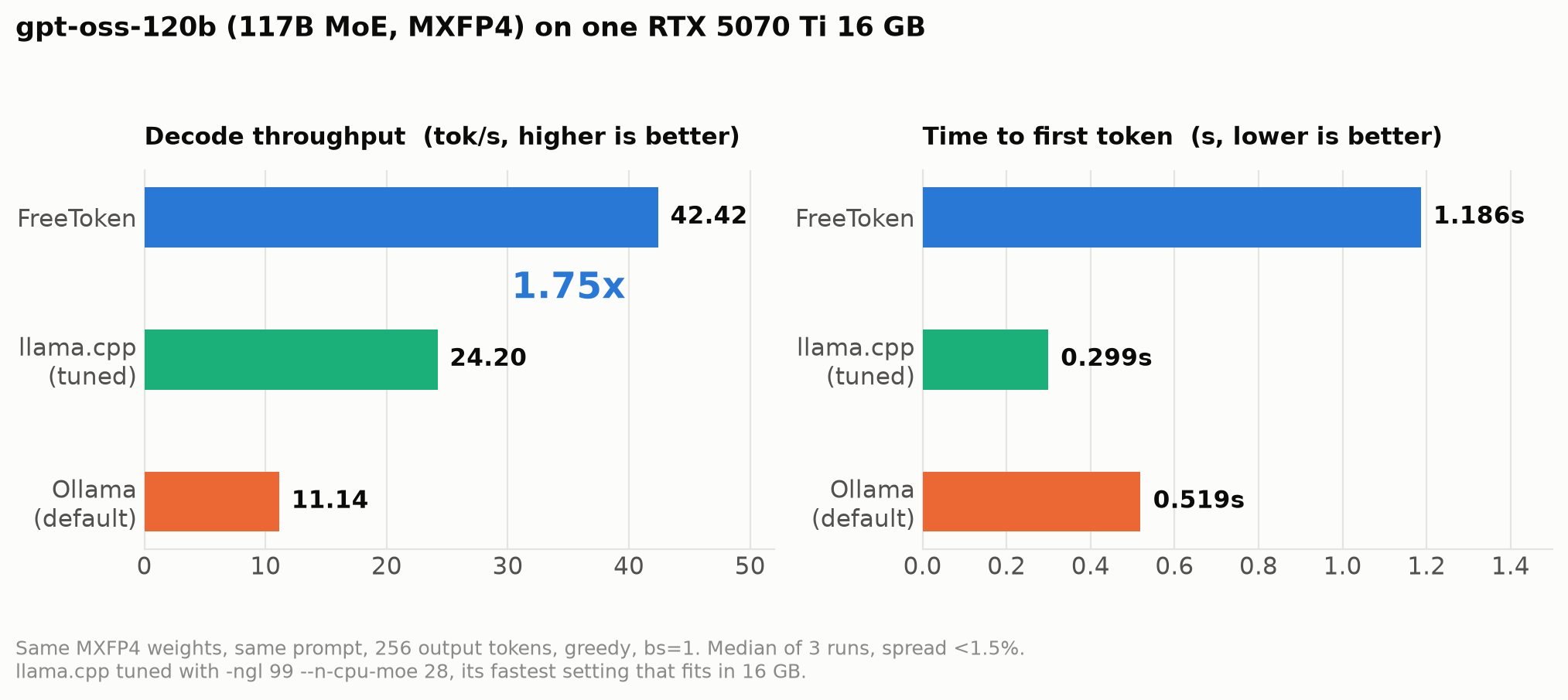
<p>One RTX 5070 Ti, 16 GB of VRAM, serving <strong>gpt-oss-120b</strong>. That’s 117 billion parameters, 61 GB of weights on disk.</p>

<p><img src="/assets/images/inference/freetoken-throughput.png" alt="Three-engine comparison" /></p>

<div class="language-text highlighter-rouge"><div class="highlight"><pre class="highlight"><code>FreeToken            42.42 tokens/s
llama.cpp (tuned)    24.20 tokens/s     1.75x slower
Ollama (default)     11.14 tokens/s     3.81x slower
</code></pre></div></div>

<p>Same MXFP4 weights in all three. Same prompt, 256 output tokens, greedy. Everything separating them is a decision about what lives where.</p>

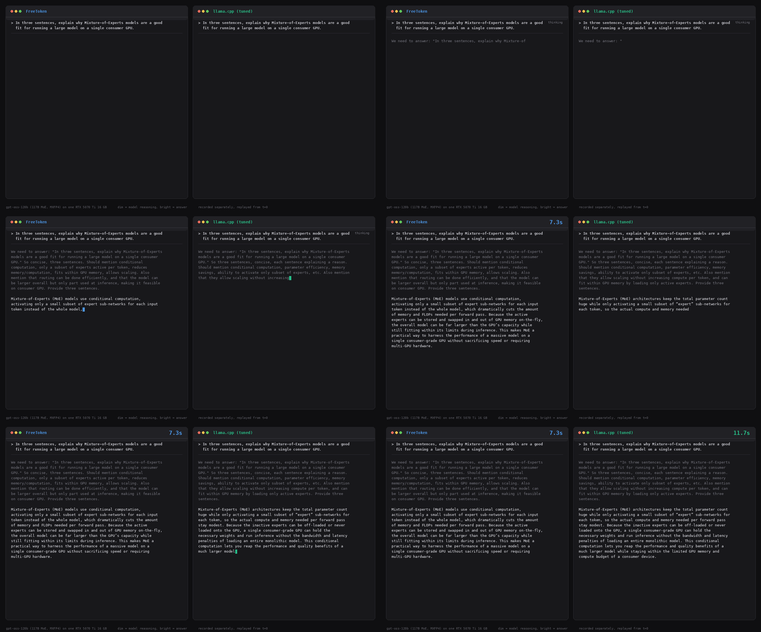
<p>Here is what that gap looks like. Both engines answering the same question, replayed at the speed they actually ran:</p>

<p><img src="/assets/images/inference/freetoken-vs-llamacpp.gif" alt="FreeToken and llama.cpp generating side by side" /></p>

<hr />

<h1 id="1-the-setup">1. The Setup</h1>

<p>An ordinary gaming desktop:</p>

<ul>
  <li><strong>GPU</strong> — RTX 5070 Ti, 16 GB VRAM, sm_120 (Blackwell)</li>
  <li><strong>CPU</strong> — Ryzen 9 9900X, 12 physical cores</li>
  <li><strong>RAM</strong> — 128 GB DDR5</li>
  <li><strong>Link</strong> — PCIe 5.0 x16</li>
  <li><strong>OS</strong> — Windows 11, everything run inside WSL2 (Ubuntu 24.04)</li>
</ul>

<p>FreeToken’s CLI is Linux-only, so WSL2 wasn’t optional. It quietly costs about 7%, and I’ll come back to that.</p>

<p>The 128 GB of system RAM is what makes this machine interesting. Expert offloading treats host memory as the model’s real home and lets the GPU borrow pieces of it, so RAM capacity sets the ceiling on what you can serve at all.</p>

<p>Picking the model took longer than expected. The README advertises 290B+ models, but I checked the actual checkpoint sizes first and most of them don’t fit in 128 GB. GLM-5.2 wants about 400 GB. DeepSeek-V4-Flash wants 167 GB. gpt-oss-120b at 65 GB was one of the few that did fit, and it had a property I cared about more than size:</p>

<blockquote>
  <p>Ollama’s <code class="language-plaintext highlighter-rouge">gpt-oss:120b</code> and the Hugging Face checkpoint are <strong>the same MXFP4 weights</strong>.</p>
</blockquote>

<p>Local inference comparisons are usually contaminated. One engine runs a 4-bit GGUF, the other runs something else, and part of the speed difference is really a precision difference nobody mentions. Here I could confirm all three engines load identical numbers, so the benchmark measures engines.</p>

<hr />

<h1 id="2-freetoken-measures-your-machine-first">2. FreeToken Measures Your Machine First</h1>

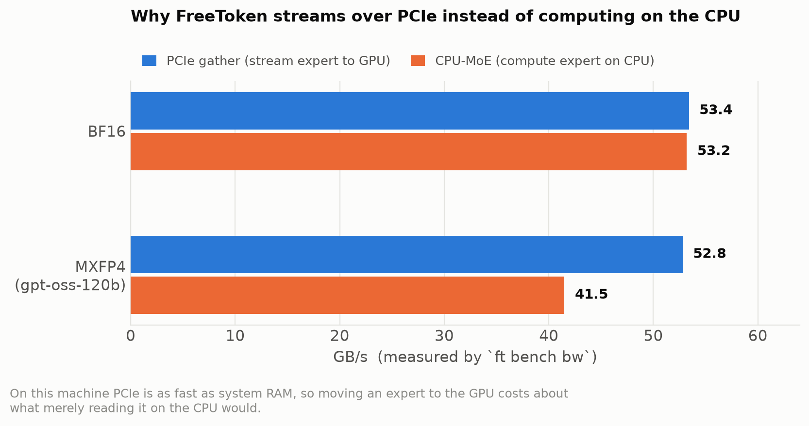
<p>Before serving anything, FreeToken runs a calibration pass over the two routes an expert can take. Copy it across PCIe to the GPU, or leave it in RAM and compute on the CPU.</p>

<div class="language-bash highlighter-rouge"><div class="highlight"><pre class="highlight"><code>ft bench bw <span class="nt">--dtype</span> mxfp4,bf16
</code></pre></div></div>

<p><img src="/assets/images/inference/freetoken-bandwidth.png" alt="CPU vs PCIe bandwidth" /></p>

<p>PCIe came in at 56.6 GB/s. The CPU’s entire memory read bandwidth is 54.2 GB/s. So shipping an expert to the GPU costs roughly what reading it on the CPU costs, before the CPU does any arithmetic at all. PCIe 5.0 is just that fast next to dual-channel DDR5.</p>

<p>FreeToken only splits work across both paths when the CPU is at least twice as fast. It isn’t close here, so it picked pure PCIe streaming:</p>

<div class="language-text highlighter-rouge"><div class="highlight"><pre class="highlight"><code>Auto-selected MoE backend: offload
</code></pre></div></div>

<p>Which means the paper’s headline mechanism, the bandwidth-adaptive split, does nothing on my hardware. That’s the policy working. Its job is to look at the machine and decide, and on a PCIe-rich desktop the right decision is to leave the CPU alone. It would earn its keep on a laptop with a narrow PCIe link, or a workstation with eight memory channels feeding a slower bus. I don’t have either, so I can only report that it declined to engage and was right.</p>

<hr />

<h1 id="3-the-first-answer-and-why-it-was-wrong">3. The First Answer, and Why It Was Wrong</h1>

<p>I started with Ollama, since that’s what most people have installed. FreeToken hit 42.42 tok/s against Ollama’s 11.14. A 3.81x gap is larger than I predicted, so I went looking for a bug in my harness instead of believing it.</p>

<p>The harness was fine. The baseline wasn’t. Running <code class="language-plaintext highlighter-rouge">ollama ps</code> during the benchmark showed what was actually happening:</p>

<div class="language-text highlighter-rouge"><div class="highlight"><pre class="highlight"><code>gpt-oss:120b   66 GB   78%/22% CPU/GPU   4096 ctx
"offloaded 8/37 layers to GPU"
</code></pre></div></div>

<p>Eight complete layers on the GPU, twenty-nine running entirely on the CPU. When I went looking for a way to improve that, I found Ollama doesn’t really offer one. Its environment variables cover context length, KV cache type, flash attention. Nothing that changes <em>how</em> the model gets split. The one offload knob is <code class="language-plaintext highlighter-rouge">num_gpu</code>, which sets how many whole layers go to the GPU, and Ollama had already filled VRAM to 14.5 of 16.3 GB. Maybe one more layer would fit.</p>

<p>“3.81x faster than Ollama” is a true measurement of a real default configuration. It is not a fair statement about the state of the art. Ollama wraps llama.cpp, and llama.cpp has a much better option that Ollama never exposes.</p>

<hr />

<h1 id="4-the-real-comparison">4. The Real Comparison</h1>

<p>The option is <code class="language-plaintext highlighter-rouge">--n-cpu-moe</code>, and why it matters is the whole point of this post.</p>

<p>A transformer layer holds two things with completely different shapes. Attention is small but does heavy math. The experts are enormous but only a handful get used per token; gpt-oss-120b has 128 per layer and picks 4. When Ollama sends a layer to the CPU it sends both. The small compute-heavy part gets dragged onto the slow device along with the bulky part, for no reason anyone would choose.</p>

<p><code class="language-plaintext highlighter-rouge">--n-cpu-moe N</code> pulls them apart. Every layer’s attention stays on the GPU, and only the expert weights of the first N layers move to the CPU. Heavy math on the fast device, bulk wherever there’s room.</p>

<p>Getting this measured was more annoying than it should have been. CUDA 13.1’s runtime segfaults inside WSL’s driver stub, so I built llama.cpp against 12.8 instead. Then Ollama’s GGUF refused to load, because it declares its architecture as <code class="language-plaintext highlighter-rouge">gptoss</code> while upstream llama.cpp expects <code class="language-plaintext highlighter-rouge">gpt-oss</code>. Ollama’s model files aren’t readable by the project it’s built on. I ended up downloading llama.cpp’s own MXFP4 build of the same model.</p>

<p>With that sorted, llama.cpp reaches <strong>24.20 tok/s</strong>. That is more than double Ollama’s 11.14, on the same engine, same weights, same GPU. One flag.</p>

<hr />

<h1 id="5-why-llamacpp-still-hits-a-ceiling">5. Why llama.cpp Still Hits a Ceiling</h1>

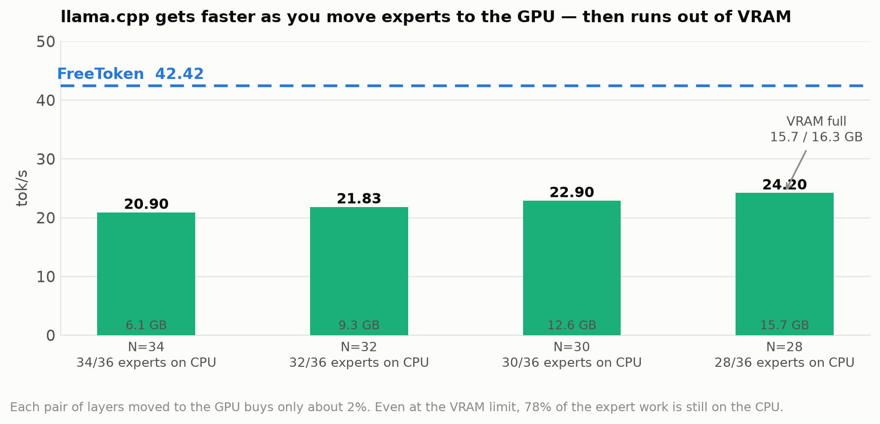
<p><img src="/assets/images/inference/freetoken-ceiling.png" alt="llama.cpp scaling" /></p>

<p>The sweep tells you more than the peak number does. Every time I moved two more layers’ worth of experts onto the GPU, throughput rose about 2%. The climb stops at N=28, with 15.7 of 16.3 GB used. There is nowhere left to go.</p>

<p>At that limit, 78% of the expert work is still on the CPU. Moving layers two at a time picks at the edge of the problem without changing it. The CPU carries the bulk either way, and it manages roughly 16 GB/s effective, under a third of what PCIe delivers here.</p>

<p>FreeToken gets 42.42 tok/s using <em>less</em> VRAM, 13.9 GB. It never makes the layer-level decision. All 36 layers compute on the GPU and individual experts get fetched across PCIe as the router asks for them. You’re moving books instead of shelves.</p>

<p>One measurement shows the payoff cleanly. FreeToken keeps recently-used experts cached in VRAM, 702 of the model’s 4,608, about 15%. If the router picked at random, that cache would hit 15% of the time. It hits 31.5%:</p>

<div class="language-text highlighter-rouge"><div class="highlight"><pre class="highlight"><code>15.2% of experts resident  -&gt;  31.5% of lookups served
</code></pre></div></div>

<p>Routers have favourites. Some experts are far more popular than others, and a cache working at expert granularity can exploit that. A layer-granularity cache can’t, because it committed to whole layers before the router said anything.</p>

<hr />

<h1 id="6-what-i-take-away">6. What I Take Away</h1>

<p>The paper’s framing held up, but not through the mechanism it spends the most pages on. The bandwidth-adaptive split sat inert on my hardware. It measured the machine, concluded the CPU wasn’t worth using, and got out of the way. The gap came from the plainer decision to offload at expert granularity rather than layer granularity, plus a cache that exploits the fact that routers have favourites.</p>

<p>That’s the part worth carrying elsewhere. A layer is a convenient unit when you’re writing the code, because it’s how the model is built. It’s a bad unit when you’re scheduling, because it forces two unrelated decisions to be made together and one of them is usually wrong.</p>

<p>The other thing I’d keep is about method. My first number was measured correctly, reproduced cleanly, and misled anyway. It only became honest after I went and built the thing I had dismissed in a caveat. When a benchmark writeup says “of course, X wasn’t tuned,” that’s usually the experiment that needed running.</p>

<hr />]]></content><author><name></name></author><category term="mlsys" /><category term="inference" /><summary type="html"><![CDATA[The last post covered the FreeToken paper, which argues that running a big MoE model locally is a scheduling problem rather than a fitting-in-VRAM problem. Fine as an argument. I wanted to know if it beats the tools I already have installed.]]></summary></entry><entry><title type="html">FreeToken: Making Large MoE Models Practical on a Single Machine</title><link href="https://minseoc03.github.io/mlsys/inference/freetoken/" rel="alternate" type="text/html" title="FreeToken: Making Large MoE Models Practical on a Single Machine" /><published>2026-08-25T08:43:00+00:00</published><updated>2026-08-25T08:43:00+00:00</updated><id>https://minseoc03.github.io/mlsys/inference/freetoken</id><content type="html" xml:base="https://minseoc03.github.io/mlsys/inference/freetoken/"><![CDATA[<blockquote>
  <p><strong>Paper:</strong> <em>FreeToken: Efficient Edge-Native MoE Serving with Bandwidth-Adaptive Execution</em><br />
<strong>arXiv:</strong> 2608.16157<br />
<strong>Link:</strong> https://arxiv.org/abs/2608.16157</p>
</blockquote>

<p>Large Mixture-of-Experts models are interesting for local inference because they are huge in total parameter count while activating only a small fraction of those parameters for each token. On paper, that sounds ideal: a 200B+ parameter MoE model may use only around 10–20B parameters per token, so the actual compute cost can be much smaller than the total model size suggests. But there is an obvious problem:</p>

<blockquote>
  <p>Even if only a few experts are active at a time, all of the expert weights still need to live somewhere.</p>
</blockquote>

<p>For consumer hardware, that usually means keeping most experts in CPU memory while only part of the model fits in GPU VRAM. <strong>FreeToken</strong> is about making this setup much more efficient, and its main idea is surprisingly simple:</p>

<blockquote>
  <p>Instead of always moving a missing expert to the GPU, or always computing it on the CPU, FreeToken uses both paths at the same time and decides the split based on the machine’s actual memory bandwidth.</p>
</blockquote>

<p>That idea is combined with different strategies for <strong>prefill</strong>, <strong>decode</strong>, <strong>expert caching</strong>, <strong>agent workloads</strong>, and <strong>GPU memory management</strong>.</p>

<hr />

<h2 id="the-core-problem">The Core Problem</h2>

<p>A typical local MoE setup looks roughly like this:</p>

<div class="language-text highlighter-rouge"><div class="highlight"><pre class="highlight"><code>                GPU
        ┌─────────────────┐
        │ Attention       │
        │ Shared layers   │
        │ Expert cache    │
        └────────┬────────┘
                 │ PCIe
                 │
        ┌────────▼────────┐
        │ CPU DRAM        │
        │ Full expert pool│
        └─────────────────┘
</code></pre></div></div>

<p>The non-expert parts of the model can stay on the GPU, while the full set of experts remains in host memory and a subset is cached in VRAM. At that point, serving performance depends heavily on how well the runtime manages three resources:</p>

<ul>
  <li>GPU compute</li>
  <li>PCIe bandwidth</li>
  <li>CPU memory bandwidth</li>
</ul>

<p>The important part is that <strong>prefill and decode behave very differently</strong>, and that distinction drives much of FreeToken’s design.</p>

<hr />

<h1 id="1-prefill-and-decode-are-different-problems">1. Prefill and Decode Are Different Problems</h1>

<p>For a single decode token, the router may only select a few experts. For example:</p>

<div class="language-text highlighter-rouge"><div class="highlight"><pre class="highlight"><code>token t
   │
   ▼
 router
   │
   ├── Expert 3
   ├── Expert 7
   ├── Expert 12
   └── Expert 18
</code></pre></div></div>

<p>This is the normal advantage of MoE: only a small subset of the model is active. But prefill is different. Suppose a prompt contains thousands of tokens. Each token may select different experts:</p>

<div class="language-text highlighter-rouge"><div class="highlight"><pre class="highlight"><code>token 1  → E1, E3
token 2  → E4, E8
token 3  → E2, E9
token 4  → E5, E11
...
token N  → E6, E10
</code></pre></div></div>

<p>Once we take the union over thousands of tokens, the model may end up touching almost every expert in the layer. So during prefill:</p>

<blockquote>
  <p><strong>MoE sparsity becomes much less useful.</strong></p>
</blockquote>

<p>This leads FreeToken to use two completely different execution strategies.</p>

<table>
  <thead>
    <tr>
      <th>Phase</th>
      <th>Main problem</th>
      <th>FreeToken’s strategy</th>
    </tr>
  </thead>
  <tbody>
    <tr>
      <td>Prefill</td>
      <td>Almost all experts are touched</td>
      <td>Stream full expert layers</td>
    </tr>
    <tr>
      <td>Decode</td>
      <td>Only a few experts are active</td>
      <td>Cache experts and handle misses dynamically</td>
    </tr>
  </tbody>
</table>

<p>This separation is one of the cleanest ideas in the paper.</p>

<hr />

<h1 id="2-prefill-stream-the-entire-layer">2. Prefill: Stream the Entire Layer</h1>

<p>During prefill, trying to predict which experts will be needed is not very useful. Instead, FreeToken assumes that most experts will eventually be used and simply streams an entire MoE layer from CPU memory to the GPU. The key optimization is <strong>double buffering</strong>. Imagine the GPU is computing layer <code class="language-plaintext highlighter-rouge">L</code>.</p>

<p>At the same time, FreeToken transfers the experts for layer <code class="language-plaintext highlighter-rouge">L+1</code>.</p>

<div class="language-text highlighter-rouge"><div class="highlight"><pre class="highlight"><code>time ─────────────────────────────────────&gt;

GPU:
[ compute layer L ]
                  [ compute layer L+1 ]
                                      [ compute layer L+2 ]

PCIe:
[ load layer L+1 ]
                  [ load layer L+2 ]
                                      [ load layer L+3 ]
</code></pre></div></div>

<p>Two buffers alternate:</p>

<div class="language-text highlighter-rouge"><div class="highlight"><pre class="highlight"><code>Buffer A → current layer

Buffer B → next layer being transferred
</code></pre></div></div>

<p>After layer <code class="language-plaintext highlighter-rouge">L</code> finishes, the buffers swap roles. In the ideal case, the execution time becomes roughly:</p>

\[T \approx \max(T_{\text{PCIe}}, T_{\text{compute}})\]

<p>instead of:</p>

\[T = T_{\text{PCIe}} + T_{\text{compute}}\]

<p>The difference is important because, instead of waiting for transfer and then computing, the runtime tries to hide one behind the other.</p>

<hr />

<h2 id="why-this-matters">Why This Matters</h2>

<p>The paper reports an experiment where an expert pool of roughly <strong>64 GB</strong> is streamed over a PCIe connection delivering around <strong>52.7 GB/s</strong>. The measured prefill time is very close to the time required to simply stream those weights once, which suggests that most of the GPU computation is effectively hidden behind the transfer. That is exactly what a good overlap-based runtime should achieve.</p>

<hr />

<h1 id="3-decode-exploit-expert-locality">3. Decode: Exploit Expert Locality</h1>

<p>Decode has a very different access pattern. A single token activates only a handful of experts, so streaming every expert would obviously be wasteful; FreeToken instead keeps an <strong>LRU expert cache</strong> inside GPU memory. The intuition is straightforward:</p>

<blockquote>
  <p>Consecutive tokens often choose similar experts.</p>
</blockquote>

<p>For example:</p>

<div class="language-text highlighter-rouge"><div class="highlight"><pre class="highlight"><code>token t-1:
E3 E7 E9 E12 E17 E24

token t:
E3 E7 E9 E12 E17 E24
</code></pre></div></div>

<p>The selection will not always be identical, but there is enough temporal locality that recently used experts are often useful again, which makes keeping these hot experts in VRAM worthwhile.</p>

<hr />

<h2 id="cache-hit">Cache Hit</h2>

<p>If the router selects an expert that already exists in the GPU cache:</p>

<div class="language-text highlighter-rouge"><div class="highlight"><pre class="highlight"><code>Router
  │
  ▼
Expert cache
  │
  └── HIT → run on GPU
</code></pre></div></div>

<p>This is the easy case. No transfer is needed.</p>

<hr />

<h2 id="cache-miss">Cache Miss</h2>

<p>The interesting part happens when an expert is not in GPU memory. A normal runtime has two obvious options.</p>

<h3 id="option-a-move-the-expert-to-the-gpu">Option A: Move the expert to the GPU</h3>

<div class="language-text highlighter-rouge"><div class="highlight"><pre class="highlight"><code>CPU DRAM
   │
   │ PCIe
   ▼
GPU VRAM
   │
   ▼
GPU compute
</code></pre></div></div>

<h3 id="option-b-keep-it-on-the-cpu">Option B: Keep it on the CPU</h3>

<div class="language-text highlighter-rouge"><div class="highlight"><pre class="highlight"><code>CPU DRAM
   │
   ▼
CPU compute
</code></pre></div></div>

<p>Many systems strongly favor one of these paths. FreeToken asks a different question:</p>

<blockquote>
  <p>Why not do both?</p>
</blockquote>

<hr />

<h1 id="4-the-most-important-idea-bandwidth-adaptive-execution">4. The Most Important Idea: Bandwidth-Adaptive Execution</h1>

<p>Suppose there are <code class="language-plaintext highlighter-rouge">m</code> missing experts for the current layer. FreeToken sends some of them to the GPU and computes the rest directly on the CPU.</p>

<div class="language-text highlighter-rouge"><div class="highlight"><pre class="highlight"><code>             Cache misses
                  │
         ┌────────┴─────────┐
         │                  │
         ▼                  ▼
   PCIe → GPU          CPU execution
</code></pre></div></div>

<p>The two paths run in parallel. The only remaining question is:</p>

<blockquote>
  <p>How many experts should go to each side?</p>
</blockquote>

<p>This is where the paper introduces its most important equation.</p>

<hr />

<h1 id="5-deriving-q">5. Deriving ($q^*$)</h1>

<p>Let:</p>

<ul>
  <li>$m$: number of cache misses</li>
  <li>$q$: number of missed experts transferred to the GPU</li>
  <li>$S$: size of one expert</li>
  <li>$B_P$: measured PCIe transfer bandwidth</li>
  <li>$B_H$: measured host-side expert processing bandwidth</li>
</ul>

<p>If <code class="language-plaintext highlighter-rouge">q</code> experts are transferred to the GPU, their transfer time is approximately:</p>

\[T_{\text{fill}}
\approx
\frac{qS}{B_P}\]

<p>The remaining:</p>

\[m-q\]

<p>experts stay on the CPU. The important observation is that PCIe DMA is also reading from host DRAM. So CPU execution and PCIe transfer compete for the same memory subsystem. FreeToken approximates the bandwidth left for CPU execution as:</p>

\[B_H-B_P\]

<p>Therefore:</p>

\[T_{\text{cpu}}
\approx
\frac{(m-q)S}{B_H-B_P}\]

<p>Because both paths execute simultaneously, the best split is approximately the point where both finish at the same time:</p>

\[T_{\text{fill}}
\approx
T_{\text{cpu}}\]

<p>So:</p>

\[\frac{qS}{B_P}
=
\frac{(m-q)S}{B_H-B_P}\]

<p>After simplifying:</p>

\[\boxed{
q^*
\approx
m\frac{B_P}{B_H}
}\]

<p>This is probably the single equation worth remembering from the paper.</p>

<hr />

<h1 id="6-a-simple-example">6. A Simple Example</h1>

<p>Suppose:</p>

\[B_H = 4\]

<p>and:</p>

\[B_P = 1\]

<p>with four cache misses:</p>

\[m=4\]

<p>Then:</p>

\[q^*
=
4\times\frac14
=
1\]

<p>So FreeToken chooses roughly:</p>

<div class="language-text highlighter-rouge"><div class="highlight"><pre class="highlight"><code>1 expert  → PCIe → GPU
3 experts → CPU execution
</code></pre></div></div>

<p>Instead of forcing all four experts onto one side, it uses both available execution paths.</p>

<hr />

<h1 id="7-why-the-policy-depends-on-the-machine">7. Why the Policy Depends on the Machine</h1>

<p>One subtle but important point is that FreeToken does <strong>not</strong> use theoretical bandwidth from hardware specifications. It measures the actual system. The paper reports machines with very different ratios between PCIe bandwidth and CPU-side expert bandwidth. For example:</p>

<table>
  <thead>
    <tr>
      <th>System</th>
      <th style="text-align: right">PCIe bandwidth (B_P)</th>
      <th style="text-align: right">Host expert bandwidth (B_H)</th>
    </tr>
  </thead>
  <tbody>
    <tr>
      <td>RTX 5090 server</td>
      <td style="text-align: right">52.7 GB/s</td>
      <td style="text-align: right">77.3 GB/s</td>
    </tr>
    <tr>
      <td>RTX 4090</td>
      <td style="text-align: right">25.1 GB/s</td>
      <td style="text-align: right">63.2 GB/s</td>
    </tr>
    <tr>
      <td>RTX 5090 desktop</td>
      <td style="text-align: right">49.0 GB/s</td>
      <td style="text-align: right">53.8 GB/s</td>
    </tr>
    <tr>
      <td>RTX 4060 laptop</td>
      <td style="text-align: right">11.8 GB/s</td>
      <td style="text-align: right">47.5 GB/s</td>
    </tr>
    <tr>
      <td>RTX PRO 6000</td>
      <td style="text-align: right">51.5 GB/s</td>
      <td style="text-align: right">178 GB/s</td>
    </tr>
  </tbody>
</table>

<p>These systems should not use the same policy. Take the RTX 4060 laptop:</p>

\[\frac{B_P}{B_H}
\approx
0.25\]

<p>If there are four cache misses:</p>

\[q^*\approx1\]

<p>So only around one expert should be transferred to the GPU. The remaining experts are better handled on the CPU. Now look at the RTX 5090 desktop:</p>

\[\frac{49}{53.8}\approx0.91\]

<p>In that case, transferring almost every missed expert to the GPU makes much more sense. This is the reason for the name:</p>

<blockquote>
  <p><strong>Bandwidth-Adaptive Execution</strong></p>
</blockquote>

<p>The runtime adapts the execution policy to the actual machine.</p>

<hr />

<h1 id="8-better-expert-caching-with-lru">8. Better Expert Caching with LRU</h1>

<p>Bandwidth-adaptive execution handles cache misses. But FreeToken first tries to reduce the number of misses in the first place. For this, it uses a global LRU expert cache. The paper reports significantly lower miss rates compared to KTransformers and llama.cpp.</p>

<p>For one Qwen model, the reported miss rates are roughly:</p>

<div class="language-text highlighter-rouge"><div class="highlight"><pre class="highlight"><code>FreeToken       16%
KTransformers   41%
llama.cpp       62%
</code></pre></div></div>

<p>For DeepSeek-V4-Flash:</p>

<div class="language-text highlighter-rouge"><div class="highlight"><pre class="highlight"><code>FreeToken       39%
KTransformers   59%
llama.cpp       89%
</code></pre></div></div>

<p>The exact numbers depend on the hardware and cache configuration, but the overall trend is clear. Dynamic locality-aware caching works better than more static placement strategies for this workload.</p>

<hr />

<h1 id="9-why-static-expert-placement-can-be-limiting">9. Why Static Expert Placement Can Be Limiting</h1>

<p>A simple MoE runtime may classify experts into two groups:</p>

<div class="language-text highlighter-rouge"><div class="highlight"><pre class="highlight"><code>GPU experts
CPU experts
</code></pre></div></div>

<p>Experts assigned to the GPU run on the GPU. Experts assigned to the CPU stay on the CPU. That is easy to implement, but it assumes expert popularity is relatively stable. FreeToken instead makes the system much more dynamic.</p>

<div class="language-text highlighter-rouge"><div class="highlight"><pre class="highlight"><code>router
   │
   ▼
GPU LRU cache
   │
   ├── hit → GPU
   │
   └── miss
          │
          ▼
      q* policy
       /     \
      /       \
 PCIe → GPU   CPU
</code></pre></div></div>

<p>The execution path can change from token to token. That makes FreeToken less like a simple CPU offloading system and more like a <strong>heterogeneous scheduler</strong>.</p>

<hr />

<h1 id="10-dynamic-scheduling-without-giving-up-cuda-graphs">10. Dynamic Scheduling Without Giving Up CUDA Graphs</h1>

<p>There is another implementation challenge. Expert routing changes every token. One token may produce:</p>

<div class="language-text highlighter-rouge"><div class="highlight"><pre class="highlight"><code>misses = {3, 8}
</code></pre></div></div>

<p>The next:</p>

<div class="language-text highlighter-rouge"><div class="highlight"><pre class="highlight"><code>misses = {2, 9, 10}
</code></pre></div></div>

<p>And the next:</p>

<div class="language-text highlighter-rouge"><div class="highlight"><pre class="highlight"><code>misses = {7}
</code></pre></div></div>

<p>A naive runtime could return to the CPU after each routing step:</p>

<div class="language-text highlighter-rouge"><div class="highlight"><pre class="highlight"><code>GPU
 ↓
CPU scheduling
 ↓
GPU
 ↓
CPU scheduling
 ↓
GPU
</code></pre></div></div>

<p>But frequent synchronization and host-side scheduling hurt decode latency. FreeToken instead performs many routing-dependent decisions directly on the GPU. The runtime handles operations such as:</p>

<ul>
  <li>expert deduplication</li>
  <li>hit/miss classification</li>
  <li>determining (q)</li>
  <li>choosing eviction victims</li>
  <li>rewriting logical expert IDs to physical cache slots</li>
</ul>

<p>without repeatedly bouncing control back to Python. The CPU-side expert work is managed by persistent native worker threads, and the system is designed to preserve CUDA Graph execution as much as possible. That implementation detail is important because the scheduling policy would not be nearly as useful if the scheduler itself introduced large per-token overhead.</p>

<hr />

<h1 id="11-dynamic-gpu-memory-management">11. Dynamic GPU Memory Management</h1>

<p>Another practical problem is VRAM allocation. GPU memory is not only used by expert weights. It also needs space for things like:</p>

<ul>
  <li>non-expert model weights</li>
  <li>KV cache</li>
  <li>temporary buffers</li>
  <li>expert cache</li>
  <li>other applications using the GPU</li>
</ul>

<p>And KV cache grows as the conversation gets longer. A static allocation might start like:</p>

<div class="language-text highlighter-rouge"><div class="highlight"><pre class="highlight"><code>Expert cache : 12 GB
KV cache     : 4 GB
</code></pre></div></div>

<p>But later the same session may need:</p>

<div class="language-text highlighter-rouge"><div class="highlight"><pre class="highlight"><code>Expert cache : 7 GB
KV cache     : 9 GB
</code></pre></div></div>

<p>FreeToken can resize the expert cache and give more VRAM to the KV cache when necessary. The full expert pool in CPU memory acts as the source of truth, so evicting or rebuilding the GPU expert cache does not affect correctness. This is a small detail compared to the main scheduling idea, but it matters a lot in a real local inference runtime.</p>

<hr />

<h1 id="12-agent-workloads-introduce-another-problem">12. Agent Workloads Introduce Another Problem</h1>

<p>The paper spends quite a bit of attention on agent workloads. That makes sense because modern agents repeatedly alternate between generation and tools. A simplified agent loop looks like:</p>

<div class="language-text highlighter-rouge"><div class="highlight"><pre class="highlight"><code>User request
    │
    ▼
LLM reasoning
    │
    ▼
Tool call
    │
    ▼
Tool result
    │
    ▼
More reasoning
    │
    ▼
Another tool call
</code></pre></div></div>

<p>The context keeps growing. At the same time, agent frameworks may rewrite or remove parts of older context. For example:</p>

<div class="language-text highlighter-rouge"><div class="highlight"><pre class="highlight"><code>system
reasoning
tool call
tool output
reasoning
tool call
...
</code></pre></div></div>

<p>Some intermediate reasoning blocks or tool outputs may be removed later. That creates a problem for prefix reuse.</p>

<hr />

<h1 id="13-semantic-aware-state-caching">13. Semantic-Aware State Caching</h1>

<p>FreeToken does not place reusable checkpoints at arbitrary token positions. Instead, it creates them at semantic boundaries such as:</p>

<div class="language-text highlighter-rouge"><div class="highlight"><pre class="highlight"><code>&lt;/think&gt;

&lt;/tool_call&gt;

&lt;/tool_output&gt;
</code></pre></div></div>

<p>The reasoning is simple. Agent frameworks usually modify context at meaningful block boundaries. So if the runtime stores state at the same kind of boundaries, there is a better chance that an old checkpoint remains reusable. For example:</p>

<div class="language-text highlighter-rouge"><div class="highlight"><pre class="highlight"><code>system
reasoning
tool call
tool output
--------------------- checkpoint
new suffix
</code></pre></div></div>

<p>If the prefix above the checkpoint is still unchanged, FreeToken only needs to recompute the new suffix. Without this mechanism:</p>

<div class="language-text highlighter-rouge"><div class="highlight"><pre class="highlight"><code>re-prefill entire context
</code></pre></div></div>

<p>With semantic state caching:</p>

<div class="language-text highlighter-rouge"><div class="highlight"><pre class="highlight"><code>reuse old state
+
prefill changed suffix
</code></pre></div></div>

<p>This becomes especially useful for long-running agent sessions.</p>

<hr />

<h1 id="14-freetoken-vs-traditional-moe-offloading">14. FreeToken vs. Traditional MoE Offloading</h1>

<p>A simplified comparison looks like this.</p>

<h2 id="static-style-offloading">Static-style offloading</h2>

<div class="language-text highlighter-rouge"><div class="highlight"><pre class="highlight"><code>Expert placement decided beforehand

GPU experts → GPU

CPU experts → CPU
</code></pre></div></div>

<p>The placement is relatively fixed.</p>

<hr />

<h2 id="freetoken">FreeToken</h2>

<div class="language-text highlighter-rouge"><div class="highlight"><pre class="highlight"><code>                     router
                       │
                       ▼
                 GPU LRU cache
                   /       \
                hit         miss
                 │            │
                 ▼            ▼
                GPU        q* policy
                           /        \
                          /          \
                  PCIe → GPU        CPU
                          \          /
                           \        /
                              merge
</code></pre></div></div>

<p>The important difference is that <strong>placement and execution are continuously adapted</strong>. An expert that ran on the CPU for one token may later be cached in the GPU. A cache miss may be transferred to the GPU on one machine but executed directly on the CPU on another machine. The hardware determines the policy.</p>

<hr />

<h1 id="15-performance-results">15. Performance Results</h1>

<p>The paper reports fairly strong decode performance on a single RTX 5090. For <strong>Qwen3.6-35B-A3B</strong>, FreeToken reaches roughly:</p>

<div class="language-text highlighter-rouge"><div class="highlight"><pre class="highlight"><code>77–83 tokens/s
</code></pre></div></div>

<p>with around a:</p>

<div class="language-text highlighter-rouge"><div class="highlight"><pre class="highlight"><code>1.8×–2.3×
</code></pre></div></div>

<p>speedup over the strongest baseline depending on the workload. For <strong>DeepSeek-V4-Flash 284B</strong>, it reaches roughly:</p>

<div class="language-text highlighter-rouge"><div class="highlight"><pre class="highlight"><code>22–25 tokens/s
</code></pre></div></div>

<p>with around:</p>

<div class="language-text highlighter-rouge"><div class="highlight"><pre class="highlight"><code>1.5×–1.9×
</code></pre></div></div>

<p>speedup over the strongest baseline. These results are interesting because the model is much larger than GPU memory. The system is not trying to make the full model fit in VRAM. It is trying to make <strong>not fitting</strong> efficient.</p>

<hr />

<h1 id="16-tail-ttft-is-especially-important-for-agents">16. Tail TTFT Is Especially Important for Agents</h1>

<p>One metric I liked in this paper is the emphasis on <strong>tail Time to First Token</strong>. For a normal chatbot, a slow request is annoying. For an agent, it can be worse. External tool clients may have timeouts.</p>

<p>A very long prefill can therefore turn into an actual system failure rather than just bad latency. The paper reports worst-case TTFT below roughly:</p>

<div class="language-text highlighter-rouge"><div class="highlight"><pre class="highlight"><code>44 seconds
</code></pre></div></div>

<p>for FreeToken across its evaluated workloads. Some baselines reached much larger values, including cases in the hundreds of seconds. This leads to a useful framing:</p>

<blockquote>
  <p>For agent systems, tail TTFT can become an availability problem.</p>
</blockquote>

<p>I think this is more meaningful than reporting only average tokens per second.</p>

<hr />

<h1 id="17-running-very-large-models-on-consumer-hardware">17. Running Very Large Models on Consumer Hardware</h1>

<p>One of the more eye-catching results is the RTX 4060 Laptop experiment. The GPU has only <strong>8 GB of VRAM</strong>, but FreeToken runs a 35B-class MoE model at around:</p>

<div class="language-text highlighter-rouge"><div class="highlight"><pre class="highlight"><code>39.3 tokens/s
</code></pre></div></div>

<p>The system obviously relies heavily on host memory, but it shows how far a good heterogeneous runtime can stretch relatively limited GPU hardware. At the other extreme, the paper runs a <strong>753B parameter model</strong> on a single RTX PRO 6000. The configuration includes:</p>

<div class="language-text highlighter-rouge"><div class="highlight"><pre class="highlight"><code>GPU VRAM : 96 GB
Host DRAM: 512 GiB
Checkpoint: ~433 GB
</code></pre></div></div>

<p>FreeToken reports around:</p>

<div class="language-text highlighter-rouge"><div class="highlight"><pre class="highlight"><code>14.9 tokens/s
</code></pre></div></div>

<p>while llama.cpp reports roughly:</p>

<div class="language-text highlighter-rouge"><div class="highlight"><pre class="highlight"><code>7.3 tokens/s
</code></pre></div></div>

<p>So “single GPU” here does <strong>not</strong> mean the entire model fits in GPU memory. It means one GPU is being combined with a very large host-memory pool. That distinction matters.</p>

<hr />

<h1 id="18-what-i-think-are-the-strongest-parts">18. What I Think Are the Strongest Parts</h1>

<p>There are a few things I particularly like about the paper.</p>

<h2 id="1-prefill-and-decode-are-treated-separately">1. Prefill and Decode Are Treated Separately</h2>

<p>This sounds obvious after reading the paper, but it is an important design decision. The access pattern is fundamentally different.</p>

<div class="language-text highlighter-rouge"><div class="highlight"><pre class="highlight"><code>Prefill
→ many tokens
→ almost every expert gets touched
→ streaming makes sense
</code></pre></div></div>

<div class="language-text highlighter-rouge"><div class="highlight"><pre class="highlight"><code>Decode
→ one or a few tokens
→ sparse expert activation
→ caching makes sense
</code></pre></div></div>

<p>Trying to force the same optimization strategy onto both phases would leave performance on the table.</p>

<hr />

<h2 id="2-the-q-policy-is-very-simple">2. The $q^*$ Policy Is Very Simple</h2>

<p>The policy boils down to:</p>

\[q^*=m\frac{B_P}{B_H}\]

<p>There is no large predictive model or complicated scheduler. It takes two measured bandwidths and uses them to balance two execution paths. Simple models are attractive in runtime systems because they are easier to understand, profile, and adapt.</p>

<hr />

<h2 id="3-it-uses-real-hardware-measurements">3. It Uses Real Hardware Measurements</h2>

<p>The paper does not assume that “PCIe 5.0 means X GB/s” or that DRAM bandwidth equals a number from a spec sheet. It profiles the actual expert workload. That matters because effective bandwidth depends on much more than the interface’s theoretical maximum.</p>

<hr />

<h2 id="4-the-paper-goes-beyond-one-isolated-optimization">4. The Paper Goes Beyond One Isolated Optimization</h2>

<p>FreeToken includes:</p>

<ul>
  <li>prefill streaming</li>
  <li>expert caching</li>
  <li>CPU/GPU scheduling</li>
  <li>CUDA Graph integration</li>
  <li>persistent CPU workers</li>
  <li>agent state caching</li>
  <li>elastic VRAM management</li>
</ul>

<p>So it feels like a runtime paper rather than a single micro-optimization.</p>

<hr />

<h1 id="19-limitations-and-things-to-keep-in-mind">19. Limitations and Things to Keep in Mind</h1>

<p>There are also a few places where I would be careful not to over-generalize the results.</p>

<h2 id="the-q-model-is-still-an-approximation">The $q^*$ Model Is Still an Approximation</h2>

<p>The model is largely bandwidth based:</p>

\[T
\approx
\frac{\text{bytes}}{\text{bandwidth}}\]

<p>That makes sense when expert execution is strongly memory bound. But CPU execution can also depend on:</p>

<ul>
  <li>SIMD efficiency</li>
  <li>quantization and dequantization</li>
  <li>NUMA behavior</li>
  <li>cache effects</li>
  <li>thread scheduling</li>
  <li>expert dimensions</li>
  <li>batch size</li>
</ul>

<p>FreeToken partly handles this by measuring effective expert bandwidth rather than using theoretical DRAM bandwidth, which is a good choice. Still, the policy may need to be re-profiled when the workload changes significantly.</p>

<hr />

<h2 id="this-is-mainly-a-small-batch-local-serving-system">This Is Mainly a Small-Batch Local Serving System</h2>

<p>The target workload is mostly:</p>

<div class="language-text highlighter-rouge"><div class="highlight"><pre class="highlight"><code>single user
interactive inference
small batches
personal machine
agent workload
</code></pre></div></div>

<p>That is very different from a datacenter inference server running continuous batching across many users. With large batches, expert reuse and scheduling behavior can change significantly. So I would not assume the exact policy transfers directly to something like a large vLLM deployment.</p>

<hr />

<h2 id="753b-on-one-gpu-needs-context">“753B on One GPU” Needs Context</h2>

<p>The paper does run a 753B model with one GPU. But that machine also has:</p>

<div class="language-text highlighter-rouge"><div class="highlight"><pre class="highlight"><code>512 GiB of host memory
</code></pre></div></div>

<p>The full checkpoint is hundreds of gigabytes. So the result demonstrates efficient <strong>GPU + CPU heterogeneous execution</strong>, not magical compression of a 753B model into 96 GB of VRAM.</p>

<hr />

<h1 id="20-the-deeper-idea-do-we-need-to-move-the-data">20. The Deeper Idea: Do We Need to Move the Data?</h1>

<p>I think this is the most interesting systems insight in the paper. A common optimization question is:</p>

<blockquote>
  <p>How can I move the weights to the GPU faster?</p>
</blockquote>

<p>FreeToken asks something slightly different:</p>

<blockquote>
  <p>Do I even need to move them?</p>
</blockquote>

<p>If an expert already lives in CPU memory, there are two possibilities:</p>

<div class="language-text highlighter-rouge"><div class="highlight"><pre class="highlight"><code>CPU memory
   │
   ├── move weights → GPU → compute
   │
   └── compute directly where the weights already are
</code></pre></div></div>

<p>Moving data is not free. Sometimes the fastest way to execute something on a GPU system is simply <strong>not to move it to the GPU</strong>. This way of thinking applies far beyond MoE models. It is a general heterogeneous-systems principle:</p>

<blockquote>
  <p>Compute placement should depend on both compute capability and data movement cost.</p>
</blockquote>

<hr />

<h1 id="21-a-better-way-to-think-about-the-paper">21. A Better Way to Think About the Paper</h1>

<p>I would not describe FreeToken simply as an “expert offloading system.” A better description is:</p>

<blockquote>
  <p><strong>FreeToken treats local MoE inference as a heterogeneous resource scheduling problem.</strong></p>
</blockquote>

<p>The runtime has to manage:</p>

<div class="language-text highlighter-rouge"><div class="highlight"><pre class="highlight"><code>GPU compute
GPU VRAM
GPU memory bandwidth
PCIe bandwidth
CPU compute
CPU DRAM bandwidth
KV cache
expert locality
agent state
</code></pre></div></div>

<p>all at the same time. The goal is not:</p>

<blockquote>
  <p>How do we fit the model on the GPU?</p>
</blockquote>

<p>The model often cannot fit. The better question is:</p>

<blockquote>
  <p>Where should every piece of computation happen, and when should its data move?</p>
</blockquote>

<p>That is a much more useful systems perspective.</p>

<hr />]]></content><author><name></name></author><category term="mlsys" /><category term="inference" /><summary type="html"><![CDATA[Paper: FreeToken: Efficient Edge-Native MoE Serving with Bandwidth-Adaptive Execution arXiv: 2608.16157 Link: https://arxiv.org/abs/2608.16157]]></summary></entry><entry><title type="html">What Happens to FlashAttention When Vera Rubin Ships?</title><link href="https://minseoc03.github.io/mlsys/hardware/fa_after_vera_rubin/" rel="alternate" type="text/html" title="What Happens to FlashAttention When Vera Rubin Ships?" /><published>2026-03-30T21:26:00+00:00</published><updated>2026-03-30T21:26:00+00:00</updated><id>https://minseoc03.github.io/mlsys/hardware/fa_after_vera_rubin</id><content type="html" xml:base="https://minseoc03.github.io/mlsys/hardware/fa_after_vera_rubin/"><![CDATA[<p>In the <a href="https://minseoc03.github.io/mlsys/hardware/flash_attention_4/">previous post</a>, we broke down how FlashAttention-4 addresses the fundamental hardware imbalance on Blackwell: tensor cores doubled to 2.25 PFLOPS for BF16, but SMEM bandwidth and MUFU throughput stayed flat. The result was a careful co-design of algorithms and kernels — polynomial exp2 emulation, conditional rescaling, 2-CTA backward passes, TMEM-aware pipelining — all targeting the specific bottlenecks that emerged when matmul got too fast for everything else.</p>

<p>Now, NVIDIA’s next-generation <strong>Vera Rubin</strong> platform is entering full production in H2 2026. The Rubin GPU packs 224 SMs (up from 148), HBM4 at 22 TB/s (2.8× Blackwell), and up to 50 PFLOPS of NVFP4 inference. Meanwhile, the Rubin CPX — a separate chip designed for massive-context processing (roughly analogous to the prefill phase in LLM serving) — delivers up to 30 PFLOPS of NVFP4 compute with 128 GB of GDDR7.</p>

<p>The question is: what happens to the attention bottleneck map? And what would a hypothetical “FlashAttention-5” need to look like?</p>

<hr />

<h2 id="the-asymmetry-gets-worse--and-multiplies">The Asymmetry Gets Worse — And Multiplies</h2>

<p>FA4’s insight was clean: one asymmetry (tensor cores 2× faster, everything else flat) → identify the shifted bottlenecks → attack each one. On Rubin, the picture is messier because multiple asymmetries stack on top of each other.</p>

<h3 id="the-numbers-we-know">The Numbers We Know</h3>

<table>
  <thead>
    <tr>
      <th> </th>
      <th>Blackwell (B200)</th>
      <th>Rubin (R200)</th>
      <th>Scaling</th>
      <th>Source</th>
    </tr>
  </thead>
  <tbody>
    <tr>
      <td>NVFP4 tensor core (dense)</td>
      <td>10 PFLOPS</td>
      <td>35 PFLOPS</td>
      <td><strong>3.5×</strong></td>
      <td>Official</td>
    </tr>
    <tr>
      <td>BF16 tensor core</td>
      <td>~2.25 PFLOPS</td>
      <td>~3.6 PFLOPS</td>
      <td><strong>~1.6×</strong></td>
      <td><em>Estimated</em>¹</td>
    </tr>
    <tr>
      <td>HBM bandwidth</td>
      <td>8 TB/s</td>
      <td>22 TB/s</td>
      <td><strong>2.8×</strong></td>
      <td>Official</td>
    </tr>
    <tr>
      <td>SM count</td>
      <td>148</td>
      <td>224</td>
      <td><strong>1.5×</strong></td>
      <td>Official</td>
    </tr>
    <tr>
      <td>NVLink bandwidth/GPU</td>
      <td>1.8 TB/s</td>
      <td>3.6 TB/s</td>
      <td><strong>2×</strong></td>
      <td>Official</td>
    </tr>
    <tr>
      <td>HBM capacity</td>
      <td>192 GB</td>
      <td>288 GB</td>
      <td><strong>1.5×</strong></td>
      <td>Official</td>
    </tr>
    <tr>
      <td>SMEM bandwidth/SM</td>
      <td>128 B/cycle</td>
      <td>?</td>
      <td><strong>?</strong></td>
      <td>Not disclosed</td>
    </tr>
    <tr>
      <td>MUFU throughput/SM</td>
      <td>16 ops/cycle</td>
      <td>?</td>
      <td><strong>?</strong></td>
      <td>Not disclosed</td>
    </tr>
  </tbody>
</table>

<p><em>¹ BF16 ~3.6 PFLOPS is a back-of-the-envelope estimate based on SM count scaling (224/148 × 2.25 ≈ 3.4) and likely clock speed improvements, not an official NVIDIA specification. NVIDIA’s public Rubin disclosures emphasize NVFP4 and FP8 performance.</em></p>

<p>The critical unknowns are SMEM bandwidth per SM and MUFU throughput per SM. NVIDIA hasn’t disclosed these for Rubin. But the pattern from Hopper → Blackwell is instructive: tensor core throughput doubled per SM, SMEM bandwidth stayed at 128 B/cycle, MUFU stayed at 16 ops/cycle. If this trend continues — even partially — the relative gap between matmul and non-matmul only widens further.</p>

<h3 id="bf16-a-modest-shift">BF16: A Modest Shift</h3>

<p>For BF16 workloads, Rubin’s tensor core scaling is relatively modest (~1.6×). If SMEM and MUFU scale similarly or slightly less, the bottleneck profile stays roughly similar to Blackwell. FA4’s existing techniques — exp2 emulation, conditional rescaling, 2-CTA SMEM reduction — should port well with minor retuning. The 224 SMs (vs 148) mean more parallelism, which helps with occupancy but doesn’t change the per-SM roofline.</p>

<p>This is the easy case.</p>

<h3 id="fp4-where-things-get-interesting">FP4: Where Things Get Interesting</h3>

<p>FP4 is where Rubin’s design intent is most visible. At 3.5× the dense NVFP4 throughput of Blackwell, and with a new Transformer Engine featuring adaptive compression that can push effective throughput toward 50 PFLOPS, the tensor cores are leaving everything else behind at an unprecedented rate.</p>

<p>Let’s sketch an FA4-style roofline analysis for a hypothetical NVFP4 attention forward pass. Under a mixed-precision regime, portions of the QK^T and PV matmuls could exploit NVFP4 tensor cores (with FP32 accumulators and scaling metadata), but the softmax — max, subtract, exponentiate, sum, normalize — typically relies on higher precision (often FP32) for numerical stability. You can’t meaningfully compute <code class="language-plaintext highlighter-rouge">exp2(x)</code> at 4-bit precision. This creates a widening gap:</p>

<ul>
  <li><strong>MMA time could drop by up to ~3.5×</strong> (if NVFP4 tensor cores are fully utilized for QK^T/PV).</li>
  <li><strong>Exponential time stays the same</strong> (MUFU is precision-agnostic for transcendentals — it always operates in FP32).</li>
  <li><strong>SMEM traffic changes modestly</strong> (NVFP4 operands are smaller, but accumulation is still FP32, and P likely needs FP8 or BF16 precision for the PV matmul).</li>
</ul>

<p>On Blackwell with BF16, the roofline showed MMA and exponential roughly tied (~1024 cycles each for 128³ tiles). With FP4 on Rubin, if MMA cycles drop by 3.5× but exponential stays flat, the exponential unit would dominate by a factor of <strong>~3.5×</strong>. The softmax wouldn’t just be a co-bottleneck — it would become the <em>overwhelming</em> bottleneck.</p>

<p>This means FA4’s current 10-25% FMA emulation split would be wildly insufficient. A Rubin-optimized FP4 attention kernel might need:</p>

<ol>
  <li><strong>50-75% FMA emulation</strong> — or whatever ratio matches the new MMA-to-MUFU throughput gap.</li>
  <li><strong>Higher-degree polynomials</strong> — FP4’s quantization error is enormous (~6% relative error), so a degree-3 polynomial is still fine. But if intermediate precision increases (e.g., FP8 softmax outputs), degree-4 or degree-5 might be needed.</li>
  <li><strong>Alternative approximation strategies</strong> — at some point, polynomial emulation on FMA units hits diminishing returns due to register pressure and latency. Lookup table–based approaches, piecewise linear approximations, or even dedicated softmax-aware hardware (which Rubin’s Transformer Engine might provide) could be the next step.</li>
</ol>

<hr />

<h2 id="the-adaptive-compression-wild-card">The Adaptive Compression Wild Card</h2>

<p>Rubin’s most architecturally novel feature for attention is the <strong>3rd-generation Transformer Engine with adaptive compression</strong>. Unlike Blackwell’s structured 2:4 sparsity (which required exactly half of values to be zero, and which almost nobody used in practice), Rubin’s adaptive compression dynamically detects and skips zeros in the data stream without forcing values to zero.</p>

<p><em>What follows is speculative — NVIDIA has not disclosed how adaptive compression interacts with fused attention kernels at the SM level. But the architectural implications are worth exploring.</em></p>

<p>One possible implication for attention: the attention matrix P = softmax(QK^T) is naturally sparse in many practical settings — especially with causal masking, local attention windows, or after the first few tokens where most attention weights are near zero. If the Transformer Engine can skip near-zero P values during the PV matmul, the effective FLOPS for PV could drop without any algorithmic change.</p>

<p>But exploiting this — if it is exposed to software at the tensor-input boundary — would likely require the FA kernel to:</p>

<ol>
  <li><strong>Produce P in a format the Transformer Engine can compress.</strong> This might mean specific memory layouts, quantization schemes, or metadata that the hardware compression can consume.</li>
  <li><strong>Coordinate compression with tiling.</strong> If compression ratios vary across tiles (dense attention regions vs. sparse regions), the pipeline timing becomes data-dependent — potentially disrupting the carefully balanced ping-pong schedules that FA4 uses.</li>
  <li><strong>Potentially rethink the softmax-to-MMA boundary.</strong> Currently, P is computed, stored to TMEM, and consumed by the PV MMA. If the compression engine operates between these stages, there might be an additional pipeline step — or it might be entirely transparent if the hardware handles it on the MMA input path.</li>
</ol>

<p>These are open design questions, not known hardware contracts. But they illustrate the kind of hardware-algorithm co-design that FA4 demonstrated is essential.</p>

<hr />

<h2 id="the-backward-pass-smem-pressure-intensifies">The Backward Pass: SMEM Pressure Intensifies</h2>

<p>FA4’s backward pass analysis showed that shared memory traffic exceeds MMA compute by ~30% in the 1-CTA case, reduced to ~5% with 2-CTA mode. On Rubin, if tensor cores get faster while per-SM SMEM bandwidth stays flat (as it did from Hopper to Blackwell — though this is not yet confirmed for Rubin), the backward pass becomes even more SMEM-dominated.</p>

<p>FA4’s 2-CTA approach halves operand B traffic by having each CTA stage only half of B. A natural extension <em>would be</em> larger cooperative MMA patterns — e.g., 4-CTA or cluster-wide operand sharing — though whether Rubin’s hardware supports this is unknown at time of writing. Blackwell’s 2-CTA mode was a new capability that didn’t exist on Hopper; Rubin may similarly introduce new cooperative primitives.</p>

<p>Similarly, if TMEM capacity increases on Rubin (not yet disclosed), more intermediate results could stay in TMEM, reducing SMEM round-trips. These are possibilities to watch for in the Rubin architecture documentation, not confirmed features.</p>

<p>The dQ atomic reduction problem also scales: with more SMs (224 vs 148), more CTAs are writing to the same dQ tiles, increasing atomic contention. The deterministic backward pass’s semaphore-based serialization becomes more expensive as the CTA count grows.</p>

<hr />

<h2 id="rubin-cpx-a-completely-different-attention-problem">Rubin CPX: A Completely Different Attention Problem</h2>

<p>The Rubin CPX is perhaps the most interesting challenge for FlashAttention. Designed for massive-context processing (the compute-heavy “context phase” roughly analogous to prefill in LLM serving), it has a radically different compute-to-bandwidth ratio compared to the R200:</p>

<table>
  <thead>
    <tr>
      <th> </th>
      <th>R200</th>
      <th>Rubin CPX</th>
      <th>Source</th>
    </tr>
  </thead>
  <tbody>
    <tr>
      <td>NVFP4 compute</td>
      <td>35 PFLOPS (dense)</td>
      <td>up to 30 PFLOPS</td>
      <td>Official</td>
    </tr>
    <tr>
      <td>Memory</td>
      <td>288 GB HBM4</td>
      <td>128 GB GDDR7</td>
      <td>Official</td>
    </tr>
    <tr>
      <td>HBM/memory bandwidth</td>
      <td>22 TB/s</td>
      <td><em>Not officially disclosed per-chip</em>²</td>
      <td>—</td>
    </tr>
    <tr>
      <td><strong>Compute/BW ratio</strong></td>
      <td>~1,590 FLOPS/byte</td>
      <td><strong>Substantially higher</strong></td>
      <td>—</td>
    </tr>
  </tbody>
</table>

<p><em>² NVIDIA discloses 1.7 PB/s memory bandwidth for the full NVL144 CPX rack (144 GPUs), but per-chip GDDR7 bandwidth has not been officially specified. Third-party estimates place it around 2 TB/s, which would imply ~10,000-15,000 FLOPS/byte — roughly 6-10× more compute-heavy than the R200. The exact ratio matters less than the directional conclusion: CPX is far more compute-dense relative to its memory bandwidth.</em></p>

<p>This extreme ratio means:</p>

<h3 id="flashattentions-io-awareness-becomes-even-more-critical">FlashAttention’s IO-Awareness Becomes Even More Critical</h3>

<p>The entire point of FlashAttention was to avoid materializing the N×N attention matrix in HBM. On CPX, with relatively limited memory bandwidth compared to its compute, even modest memory traffic is costly. The tiling strategy must be even more aggressive — larger tiles to maximize compute per byte loaded, potentially at the cost of more TMEM/register pressure.</p>

<h3 id="recomputation-becomes-freeer">Recomputation Becomes Free(er)</h3>

<p>On CPX, compute is abundant relative to bandwidth. FlashAttention already recomputes S = QK^T in the backward pass rather than storing it. On CPX, you could afford to recompute even more aggressively — for example, recomputing partial softmax results rather than storing statistics, or computing QK^T multiple times with different tile decompositions to optimize memory access patterns.</p>

<h3 id="the-kernel-architecture-might-invert">The Kernel Architecture Might Invert</h3>

<p>On the R200, FA4 tries to keep the tensor cores busy and hide SMEM/MUFU latency. On CPX, the tensor cores have so much throughput relative to memory bandwidth that the kernel might be <strong>memory-bound even with FlashAttention’s tiling</strong>. In this regime, the optimization target flips: instead of “keep tensor cores busy,” it becomes “minimize every byte of memory traffic, even if tensor cores idle.” This might mean:</p>

<ul>
  <li><strong>Longer inner loops</strong> (process more KV blocks before writing back) to amortize the cost of loading Q.</li>
  <li><strong>Fused QKV loading</strong> — loading Q, K, V in a single TMA operation rather than separate stages.</li>
  <li><strong>KV cache compression in-flight</strong> — if the Transformer Engine can decompress KV cache on the fly during the MMA, the effective memory bandwidth for loading K and V increases.</li>
</ul>

<p>This is essentially a <strong>different kernel for the same algorithm</strong> — same FlashAttention math, but with the pipeline optimized for a completely different hardware profile.</p>

<hr />

<h2 id="million-token-context-rack-scale-attention">Million-Token Context: Rack-Scale Attention</h2>

<p>Vera Rubin NVL72 connects 72 GPUs with NVLink 6 at 3.6 TB/s per GPU. With 288 GB HBM per GPU, the total memory pool is 20.7 TB — enough for million-token contexts with large KV caches.</p>

<p>But million-token attention means N = 1,000,000, and even with FlashAttention’s linear memory, the <em>compute</em> scales as O(N²). At some point, the KV cache for a single head doesn’t fit on one GPU, and attention becomes a <strong>distributed problem</strong>.</p>

<p>Current approaches (like Ring Attention and sequence parallelism) tile the sequence across GPUs and overlap communication with computation. But the FA4-style roofline analysis hasn’t been applied to the distributed case. The relevant “feeds and speeds” expand to include:</p>

<ul>
  <li><strong>NVLink bandwidth</strong> (3.6 TB/s) for moving KV blocks between GPUs</li>
  <li><strong>NVLink latency</strong> for synchronizing softmax statistics across sequence partitions</li>
  <li><strong>Load balancing</strong> across GPUs when causal masking makes some partitions much heavier than others</li>
</ul>

<p>An FA5 for Rubin might need to co-design the <strong>intra-SM pipeline</strong> (tile-level, as FA4 does) with the <strong>inter-GPU communication schedule</strong> (sequence-level). The LPT scheduling that FA4 applies within a single GPU could extend to scheduling across GPUs — placing the heaviest sequence partitions on GPUs that finish their local work first.</p>

<hr />

<h2 id="the-framework-advantage">The Framework Advantage</h2>

<p>Here’s where FA4’s most practical contribution — the CuTe-DSL framework — pays compound dividends. Adapting attention kernels to Rubin’s new hardware requires rapid experimentation:</p>

<ul>
  <li>Tuning the FMA/MUFU emulation ratio for each precision (FP4, FP8, BF16).</li>
  <li>Exploring new tile sizes and pipeline stages for the different compute/bandwidth ratios (R200 vs CPX).</li>
  <li>Integrating with the new Transformer Engine’s adaptive compression APIs.</li>
  <li>Prototyping cluster-wide MMA patterns (4-CTA or beyond).</li>
</ul>

<p>In the FA3 era, each such experiment required modifying C++ templates and waiting 55 seconds per compile. With CuTe-DSL’s 2.5-second JIT compilation, a researcher can iterate 20× faster. This isn’t just a convenience — it fundamentally changes what’s practical to explore.</p>

<p>The modular design also helps: the block-sparse, masking, and scheduling primitives are orthogonal, so adapting to Rubin’s new features (adaptive compression, larger clusters) can be done by adding new primitives without rewriting the core softmax or MMA logic.</p>

<hr />

<h2 id="summary-the-bottleneck-multiplication-table">Summary: The Bottleneck Multiplication Table</h2>

<table>
  <thead>
    <tr>
      <th>Bottleneck</th>
      <th>Blackwell (FA4)</th>
      <th>Rubin R200 (BF16)</th>
      <th>Rubin R200 (FP4)</th>
      <th>Rubin CPX</th>
    </tr>
  </thead>
  <tbody>
    <tr>
      <td><strong>Tensor core</strong></td>
      <td>Co-bottleneck</td>
      <td>Moderate</td>
      <td>Fast</td>
      <td>Very fast</td>
    </tr>
    <tr>
      <td><strong>MUFU (exp)</strong></td>
      <td>Co-bottleneck</td>
      <td>Similar</td>
      <td><strong>Dominant</strong></td>
      <td><strong>Dominant</strong></td>
    </tr>
    <tr>
      <td><strong>SMEM bandwidth</strong></td>
      <td>Bwd bottleneck</td>
      <td>Worse</td>
      <td>Much worse</td>
      <td>Less relevant</td>
    </tr>
    <tr>
      <td><strong>HBM bandwidth</strong></td>
      <td>Not bottleneck</td>
      <td>Not bottleneck</td>
      <td>Not bottleneck</td>
      <td><strong>Dominant</strong></td>
    </tr>
    <tr>
      <td><strong>Cross-GPU comm</strong></td>
      <td>N/A</td>
      <td>Long context</td>
      <td>Long context</td>
      <td>Depends on disaggregated serving topology</td>
    </tr>
  </tbody>
</table>

<p>FA4 addressed a single clean asymmetry. On Rubin, the attention kernel faces <strong>multiple simultaneous asymmetries</strong> that vary by precision (FP4 vs BF16), chip variant (R200 vs CPX), and scale (single GPU vs rack). The methodology — roofline analysis per resource, targeted algorithmic mitigation — remains sound. But the number of configurations to optimize explodes.</p>

<p>The good news: FA4’s CuTe-DSL framework, modular primitives, and tuning infrastructure were designed for exactly this kind of rapid adaptation. The question isn’t whether the attention algorithm can keep up with the hardware. It’s whether the iteration speed of the framework can keep up with the proliferation of hardware targets.</p>

<p>If the Hopper → Blackwell transition is any guide, the answer is that the first team to have working, optimized kernels on new silicon wins — and then everyone else (including NVIDIA’s own cuDNN team) converges on the same techniques. FA4 demonstrated this pattern. On Rubin, the race starts again.</p>]]></content><author><name></name></author><category term="mlsys" /><category term="hardware" /><summary type="html"><![CDATA[FlashAttention-4 solved Blackwell's asymmetric scaling. Vera Rubin will introduce several new asymmetries — all at once.]]></summary></entry><entry><title type="html">FlashAttention-4: When Tensor Cores Got Too Fast for Everything Else</title><link href="https://minseoc03.github.io/mlsys/hardware/flash_attention_4/" rel="alternate" type="text/html" title="FlashAttention-4: When Tensor Cores Got Too Fast for Everything Else" /><published>2026-03-30T20:43:00+00:00</published><updated>2026-03-30T20:43:00+00:00</updated><id>https://minseoc03.github.io/mlsys/hardware/flash_attention_4</id><content type="html" xml:base="https://minseoc03.github.io/mlsys/hardware/flash_attention_4/"><![CDATA[<p>Every generation of GPU hardware promises faster matrix multiplication. Blackwell delivers on that promise — doubling tensor core throughput to 2.25 PFLOPS for BF16 compared to Hopper’s 1 PFLOP. But here’s the twist: <strong>everything else stayed roughly the same.</strong> Shared memory bandwidth? Unchanged. Exponential unit throughput? Unchanged. The result is a fundamentally lopsided machine where the matmul engine is screaming ahead while the rest of the chip struggles to keep up.</p>

<p>FlashAttention-4, from Tri Dao’s group at Princeton (with collaborators at Meta, Colfax Research, and NVIDIA), is the response to this new reality. Rather than porting FlashAttention-3’s Hopper-optimized kernels forward — which would either leave performance on the table or simply not compile — FA4 rebuilds from scratch around Blackwell’s actual bottlenecks. The results: up to 1613 TFLOPS/s on B200 (71% utilization), 1.3× faster than cuDNN 9.13, and 2.7× faster than Triton.</p>

<p>Let’s break down what changed and why.</p>

<hr />

<h2 id="the-problem-asymmetric-hardware-scaling">The Problem: Asymmetric Hardware Scaling</h2>

<p>On Hopper (H100), the performance balance between tensor cores, shared memory, and special function units was tight enough that a well-pipelined kernel could keep most resources busy. On Blackwell (B200), that balance is shattered.</p>

<p>Here are the numbers per SM per clock cycle:</p>

<table>
  <thead>
    <tr>
      <th>Resource</th>
      <th>Hopper (H100)</th>
      <th>Blackwell (B200)</th>
      <th>Scaling</th>
    </tr>
  </thead>
  <tbody>
    <tr>
      <td>Tensor core (BF16 MMA)</td>
      <td>4,096 ops</td>
      <td>8,192 ops</td>
      <td><strong>2×</strong></td>
    </tr>
    <tr>
      <td>Shared memory bandwidth</td>
      <td>128 bytes</td>
      <td>128 bytes</td>
      <td><strong>1×</strong></td>
    </tr>
    <tr>
      <td>Exponential unit (MUFU)</td>
      <td>16 ops</td>
      <td>16 ops</td>
      <td><strong>1×</strong></td>
    </tr>
  </tbody>
</table>

<p>The implication is stark. On Hopper, the attention kernel was roughly compute-bound — the bottleneck was tensor core throughput. On Blackwell, the bottleneck has shifted to <strong>shared memory traffic</strong> and <strong>exponential unit throughput</strong>. The roofline analysis in the paper confirms this: for a typical 128³ tile configuration, SMEM and exponential each take ~1024 cycles while MMA also takes ~1024 cycles. They’re neck-and-neck. But for larger tiles (256 × 128²), MMA and exponential both take 2048 cycles — meaning the kernel now has <em>two</em> co-dominant bottlenecks that are no longer matmul.</p>

<p>The forward pass bottleneck is the exponential unit. The backward pass bottleneck is shared memory bandwidth, exceeding MMA compute time by ~30%.</p>

<hr />

<h2 id="whats-new-in-blackwell-hardware">What’s New in Blackwell Hardware</h2>

<p>Before diving into the algorithmic fixes, it’s worth understanding the new hardware primitives that FA4 exploits.</p>

<h3 id="tensor-memory-tmem">Tensor Memory (TMEM)</h3>

<p>Blackwell introduces <strong>256 KB of tensor memory per SM</strong> — a new level in the memory hierarchy specifically coupled to the tensor cores. On Hopper, MMA results were written back to registers, which created enormous register pressure and limited tile sizes. On Blackwell, MMA outputs go directly to TMEM, asynchronously. This is a game-changer for two reasons:</p>

<ol>
  <li><strong>Register pressure relief.</strong> Intermediate accumulator values no longer consume the limited 256-register-per-thread budget.</li>
  <li><strong>Decoupled execution.</strong> Since MMA writes to TMEM are fully async, the tensor cores don’t block on register writeback, enabling better overlap with other operations.</li>
</ol>

<p>TMEM is allocated in 32-column (16 KB) granules and requires explicit programmer management — it’s not a transparent cache.</p>

<h3 id="larger-tile-sizes">Larger Tile Sizes</h3>

<p>Blackwell MMA instructions operate on <strong>128 × 128</strong> tiles (doubled from Hopper’s 64 × 128). This means fewer instructions per output tile, but also that each instruction touches more shared memory — amplifying the SMEM bandwidth bottleneck.</p>

<h3 id="2-cta-mma-mode">2-CTA MMA Mode</h3>

<p>Blackwell supports a cooperative mode where two CTAs within a cluster jointly execute a single MMA. The accumulator is partitioned along the M dimension, and — critically — each CTA only stages <strong>half</strong> of operand B in its shared memory while the hardware consumes the combined B tile. This effectively halves redundant SMEM traffic for operand B.</p>

<hr />

<h2 id="fix-1-redesigned-pipeline-for-mma--softmax-overlap">Fix #1: Redesigned Pipeline for MMA &amp; Softmax Overlap</h2>

<h3 id="the-core-idea">The Core Idea</h3>

<p>Since softmax computation (exponentials, max, normalization) is now a co-bottleneck with MMA, the pipeline must be designed so that <strong>while one tile’s MMA is running, another tile’s softmax is being computed</strong> — and vice versa. FA4 uses a <strong>ping-pong schedule</strong> (similar in spirit to FA3) where two output tiles are computed per thread block, but the implementation is fundamentally different due to Blackwell’s TMEM and larger tiles.</p>

<h3 id="fa3-vs-fa4-thread-assignment">FA3 vs FA4: Thread Assignment</h3>

<p>On Hopper (FA3), each row of an accumulator tile was distributed across <strong>4 threads in an interleaved pattern</strong>. Computing a row-wise operation like softmax required <strong>inter-warp shuffles</strong> — threads had to exchange partial results to reconstruct full rows before computing the row max and row sum. This shuffle overhead was a tax on every softmax step.</p>

<!-- 🔄 CHANGED: Added FA3 code snippet showing quad_allreduce shuffle -->

<p>Here’s how FA3 handles it in C++ — notice the <code class="language-plaintext highlighter-rouge">quad_allreduce_</code> call that performs cross-thread reduction, required because each thread only holds a partial row:</p>

<div class="language-cpp highlighter-rouge"><div class="highlight"><pre class="highlight"><code><span class="c1">// FA3 (Hopper) — hopper/softmax.h</span>
<span class="c1">// Each thread holds a partial row. 4 threads per row in interleaved layout.</span>
<span class="c1">// After computing local row_sum, must shuffle across threads to get the full sum.</span>

<span class="n">__forceinline__</span> <span class="n">__device__</span> <span class="n">TensorT</span> <span class="nf">finalize</span><span class="p">(</span><span class="kt">float</span> <span class="k">const</span> <span class="n">final_scale</span><span class="o">=</span><span class="mf">1.</span><span class="n">f</span><span class="p">)</span> <span class="p">{</span>
    <span class="n">SumOp</span><span class="o">&lt;</span><span class="kt">float</span><span class="o">&gt;</span> <span class="n">sum_op</span><span class="p">;</span>
    <span class="n">quad_allreduce_</span><span class="p">(</span><span class="n">row_sum</span><span class="p">,</span> <span class="n">row_sum</span><span class="p">,</span> <span class="n">sum_op</span><span class="p">);</span>  <span class="c1">// ← Cross-thread shuffle required!</span>
    <span class="n">TensorT</span> <span class="n">scores_scale</span><span class="p">;</span>
    <span class="cp">#pragma unroll
</span>    <span class="k">for</span> <span class="p">(</span><span class="kt">int</span> <span class="n">mi</span> <span class="o">=</span> <span class="mi">0</span><span class="p">;</span> <span class="n">mi</span> <span class="o">&lt;</span> <span class="n">size</span><span class="p">(</span><span class="n">row_sum</span><span class="p">);</span> <span class="o">++</span><span class="n">mi</span><span class="p">)</span> <span class="p">{</span>
        <span class="kt">float</span> <span class="n">sum</span> <span class="o">=</span> <span class="n">row_sum</span><span class="p">(</span><span class="n">mi</span><span class="p">);</span>
        <span class="kt">float</span> <span class="n">inv_sum</span> <span class="o">=</span> <span class="p">(</span><span class="n">sum</span> <span class="o">==</span> <span class="mf">0.</span><span class="n">f</span> <span class="o">||</span> <span class="n">sum</span> <span class="o">!=</span> <span class="n">sum</span><span class="p">)</span> <span class="o">?</span> <span class="mf">0.</span><span class="n">f</span> <span class="o">:</span> <span class="mf">1.</span><span class="n">f</span> <span class="o">/</span> <span class="n">sum</span><span class="p">;</span>
        <span class="n">scores_scale</span><span class="p">(</span><span class="n">mi</span><span class="p">)</span> <span class="o">=</span> <span class="n">inv_sum</span> <span class="o">*</span> <span class="n">final_scale</span><span class="p">;</span>
    <span class="p">}</span>
    <span class="k">return</span> <span class="n">scores_scale</span><span class="p">;</span>
<span class="p">};</span>
</code></pre></div></div>

<p>On Blackwell (FA4), the 128×128 tile and TMEM layout allow <strong>each thread to own an entire row of 128 elements</strong>. Two warpgroups of 128 threads each handle softmax, with each thread processing one complete row. This eliminates inter-warp shuffles entirely:</p>

<!-- 🔄 CHANGED: Added FA4 code snippet showing no-shuffle softmax -->

<div class="language-python highlighter-rouge"><div class="highlight"><pre class="highlight"><code><span class="c1"># FA4 (Blackwell) — flash_attn/cute/softmax.py
# Each thread owns an entire row → no shuffle needed.
# SoftmaxSm100 operates on 1 row per thread (num_rows=1).
</span>
<span class="o">@</span><span class="nb">staticmethod</span>
<span class="k">def</span> <span class="nf">create</span><span class="p">(</span>
    <span class="n">scale_log2</span><span class="p">:</span> <span class="n">Float32</span><span class="p">,</span>
    <span class="n">rescale_threshold</span><span class="p">:</span> <span class="n">cutlass</span><span class="p">.</span><span class="n">Constexpr</span><span class="p">[</span><span class="nb">float</span><span class="p">]</span> <span class="o">=</span> <span class="mf">0.0</span><span class="p">,</span>
    <span class="n">softmax_scale</span><span class="p">:</span> <span class="n">Float32</span> <span class="o">|</span> <span class="bp">None</span> <span class="o">=</span> <span class="bp">None</span><span class="p">,</span>
<span class="p">):</span>
    <span class="n">num_rows</span> <span class="o">=</span> <span class="mi">1</span>  <span class="c1"># ← Each thread owns exactly 1 full row. No shuffle.
</span>    <span class="n">arch</span> <span class="o">=</span> <span class="mi">100</span>
    <span class="n">row_max</span> <span class="o">=</span> <span class="n">cute</span><span class="p">.</span><span class="n">make_rmem_tensor</span><span class="p">(</span><span class="n">num_rows</span><span class="p">,</span> <span class="n">Float32</span><span class="p">)</span>
    <span class="n">row_sum</span> <span class="o">=</span> <span class="n">cute</span><span class="p">.</span><span class="n">make_rmem_tensor</span><span class="p">(</span><span class="n">num_rows</span><span class="p">,</span> <span class="n">Float32</span><span class="p">)</span>
    <span class="k">return</span> <span class="n">SoftmaxSm100</span><span class="p">(</span>
        <span class="n">scale_log2</span><span class="p">,</span> <span class="n">num_rows</span><span class="p">,</span> <span class="n">row_max</span><span class="p">,</span> <span class="n">row_sum</span><span class="p">,</span> <span class="n">arch</span><span class="p">,</span> <span class="n">softmax_scale</span><span class="p">,</span>
        <span class="n">rescale_threshold</span><span class="o">=</span><span class="n">rescale_threshold</span><span class="p">,</span>
    <span class="p">)</span>
</code></pre></div></div>

<p>The difference is structural: FA3’s <code class="language-plaintext highlighter-rouge">kNRows</code> is typically 4–8 (partial rows distributed across threads), requiring <code class="language-plaintext highlighter-rouge">quad_allreduce_</code> at finalization. FA4’s <code class="language-plaintext highlighter-rouge">num_rows = 1</code> means each thread computes the complete row max and row sum locally — zero cross-thread communication.</p>

<h3 id="decoupled-rescaling-via-correction-warpgroup">Decoupled Rescaling via Correction Warpgroup</h3>

<p>In FA3, the online softmax rescaling step — where previous output tiles are multiplied by <code class="language-plaintext highlighter-rouge">exp(m_old - m_new)</code> to account for updated row maxima — happened inline within the softmax warpgroup. This put rescaling squarely on the <strong>critical path</strong>.</p>

<!-- 🔄 CHANGED: Added FA3 rescaling code snippet -->

<div class="language-cpp highlighter-rouge"><div class="highlight"><pre class="highlight"><code><span class="c1">// FA3 (Hopper) — hopper/softmax.h</span>
<span class="c1">// Rescaling happens inline in the same warpgroup that computes softmax.</span>
<span class="c1">// This is on the critical path — must complete before the next MMA.</span>

<span class="k">template</span><span class="o">&lt;</span><span class="k">typename</span> <span class="nc">Tensor1</span><span class="p">&gt;</span>
<span class="n">__forceinline__</span> <span class="n">__device__</span> <span class="kt">void</span> <span class="nf">rescale_o</span><span class="p">(</span><span class="n">Tensor1</span> <span class="o">&amp;</span><span class="n">acc_o</span><span class="p">,</span> <span class="n">TensorT</span> <span class="k">const</span> <span class="o">&amp;</span><span class="n">scores_scale</span><span class="p">)</span> <span class="p">{</span>
    <span class="n">Tensor</span> <span class="n">acc_o_rowcol</span> <span class="o">=</span> <span class="n">make_tensor</span><span class="p">(</span><span class="n">acc_o</span><span class="p">.</span><span class="n">data</span><span class="p">(),</span>
        <span class="n">flash</span><span class="o">::</span><span class="n">convert_layout_acc_rowcol</span><span class="p">(</span><span class="n">acc_o</span><span class="p">.</span><span class="n">layout</span><span class="p">()));</span>
    <span class="cp">#pragma unroll
</span>    <span class="k">for</span> <span class="p">(</span><span class="kt">int</span> <span class="n">mi</span> <span class="o">=</span> <span class="mi">0</span><span class="p">;</span> <span class="n">mi</span> <span class="o">&lt;</span> <span class="n">size</span><span class="o">&lt;</span><span class="mi">0</span><span class="o">&gt;</span><span class="p">(</span><span class="n">acc_o_rowcol</span><span class="p">);</span> <span class="o">++</span><span class="n">mi</span><span class="p">)</span> <span class="p">{</span>
        <span class="cp">#pragma unroll
</span>        <span class="k">for</span> <span class="p">(</span><span class="kt">int</span> <span class="n">ni</span> <span class="o">=</span> <span class="mi">0</span><span class="p">;</span> <span class="n">ni</span> <span class="o">&lt;</span> <span class="n">size</span><span class="o">&lt;</span><span class="mi">1</span><span class="o">&gt;</span><span class="p">(</span><span class="n">acc_o_rowcol</span><span class="p">);</span> <span class="o">++</span><span class="n">ni</span><span class="p">)</span> <span class="p">{</span>
            <span class="n">acc_o_rowcol</span><span class="p">(</span><span class="n">mi</span><span class="p">,</span> <span class="n">ni</span><span class="p">)</span> <span class="o">*=</span> <span class="n">scores_scale</span><span class="p">(</span><span class="n">mi</span><span class="p">);</span>  <span class="c1">// ← On the critical path</span>
        <span class="p">}</span>
    <span class="p">}</span>
<span class="p">};</span>
</code></pre></div></div>

<p>In FA4, because intermediate results are communicated via TMEM rather than registers, the rescaling is offloaded to a separate <strong>“correction” warpgroup</strong>. The softmax warpgroups compute P and hand off rescale statistics through TMEM; the correction warpgroup applies the rescaling independently. This takes rescaling off the critical path of the main softmax + MMA pipeline.</p>

<!-- 🔄 CHANGED: Added explanation of why TMEM enables decoupling -->

<p>The key enabler is TMEM: on Hopper, accumulators live in registers which are thread-private — there’s no way for a separate warpgroup to access another warpgroup’s accumulator. On Blackwell, accumulators live in TMEM which is accessible by all warpgroups within the same SM. This allows the correction warpgroup to read rescale statistics and apply them to the output accumulator independently.</p>

<p>The overall warpgroup assignment per thread block:</p>

<table>
  <thead>
    <tr>
      <th>Warpgroup</th>
      <th>Role</th>
    </tr>
  </thead>
  <tbody>
    <tr>
      <td>WG0</td>
      <td>Tensor core driver + TMA (data movement)</td>
    </tr>
    <tr>
      <td>WG1</td>
      <td>Softmax (tile H — “high” Q tile)</td>
    </tr>
    <tr>
      <td>WG2</td>
      <td>Softmax (tile L — “low” Q tile)</td>
    </tr>
    <tr>
      <td>WG3</td>
      <td>Correction (rescaling)</td>
    </tr>
  </tbody>
</table>

<!-- 🔄 CHANGED: Added FA3 warpgroup assignment comparison -->

<p>Compare with FA3’s warp specialization, where the division was simpler:</p>

<div class="language-cpp highlighter-rouge"><div class="highlight"><pre class="highlight"><code><span class="c1">// FA3 (Hopper) — hopper/flash_fwd_kernel_sm90.h</span>
<span class="c1">// Warp group 0 = Producer (TMA loads), Warp groups 1+ = Consumer (MMA + softmax)</span>
<span class="c1">// Softmax and rescaling happen in the SAME consumer warpgroup.</span>

<span class="n">pipeline_params_k</span><span class="p">.</span><span class="n">role</span> <span class="o">=</span> <span class="n">warp_group_idx</span> <span class="o">==</span> <span class="mi">0</span>
    <span class="o">?</span> <span class="n">MainloopPipelineK</span><span class="o">::</span><span class="n">ThreadCategory</span><span class="o">::</span><span class="n">Producer</span>   <span class="c1">// WG0: data movement</span>
    <span class="o">:</span> <span class="n">MainloopPipelineK</span><span class="o">::</span><span class="n">ThreadCategory</span><span class="o">::</span><span class="n">Consumer</span><span class="p">;</span>   <span class="c1">// WG1+: MMA + softmax + rescaling</span>

<span class="k">if</span> <span class="p">(</span><span class="n">warp_group_idx</span> <span class="o">==</span> <span class="mi">0</span><span class="p">)</span> <span class="p">{</span>  <span class="c1">// Producer</span>
    <span class="n">cutlass</span><span class="o">::</span><span class="n">arch</span><span class="o">::</span><span class="n">warpgroup_reg_dealloc</span><span class="o">&lt;</span><span class="n">LoadRegisterRequirement</span><span class="o">&gt;</span><span class="p">();</span>
    <span class="c1">// ... TMA loads only</span>
<span class="p">}</span> <span class="k">else</span> <span class="p">{</span>  <span class="c1">// Consumer — does EVERYTHING: MMA, softmax, rescaling</span>
    <span class="n">cutlass</span><span class="o">::</span><span class="n">arch</span><span class="o">::</span><span class="n">warpgroup_reg_alloc</span><span class="o">&lt;</span><span class="n">MmaRegisterRequirement</span><span class="o">&gt;</span><span class="p">();</span>
    <span class="c1">// ... MMA + softmax + rescale_o all interleaved in one warpgroup</span>
<span class="p">}</span>
</code></pre></div></div>

<p>FA4 splits the consumer into three specialized roles (softmax-H, softmax-L, correction), enabled by TMEM making the accumulator accessible across warpgroups.</p>

<p>The two softmax warpgroups are explicitly synchronized so their exponential-heavy critical sections don’t overlap, ensuring they don’t fight for the same MUFU resource.</p>

<h3 id="tmem-partitioning-strategy">TMEM Partitioning Strategy</h3>

<p>With 256 KB of TMEM per SM, the allocation must be carefully planned:</p>

<p><strong>Mandatory:</strong> Two output tiles (O^H, O^L) for the ping-pong schedule. At head dimension 128 with FP32 accumulators, each output tile is 128 × 128 × 4 bytes = 64 KB, so two tiles consume 128 KB — exactly half.</p>

<p><strong>Remaining 128 KB</strong> can store either:</p>
<ul>
  <li><strong>Option A:</strong> 1 S tile (FP32, 64 KB) + 2 P tiles (BF16, 32 KB each) = 128 KB</li>
  <li><strong>Option B:</strong> 2 S tiles (FP32, 64 KB each) = 128 KB, with P overwriting S in-place</li>
</ul>

<p>FA4 chooses <strong>Option B</strong>. Why?</p>

<ul>
  <li><strong>Immediate compute start.</strong> Two S tiles can be computed back-to-back at pipeline startup, filling the pipeline faster.</li>
  <li><strong>In-place conversion.</strong> Once S is consumed by softmax and converted to P (which is BF16, half the size), P overwrites S. This is safe because S is no longer needed after softmax.</li>
  <li><strong>Statistics storage.</strong> The leftover space (since P is smaller than S) is used to store rescale statistics for the correction warpgroup.</li>
  <li><strong>And two S tiles can be computed at once</strong>, immediately kicking off the pipeline.</li>
</ul>

<!-- 🔄 CHANGED: Added FA4 TMEM allocation code -->

<p>In the actual code, you can see the TMEM capacity check and 2-CTA tile configuration:</p>

<div class="language-python highlighter-rouge"><div class="highlight"><pre class="highlight"><code><span class="c1"># FA4 (Blackwell) — flash_attn/cute/flash_fwd_sm100.py
# TMEM capacity validation and tile configuration
</span>
<span class="bp">self</span><span class="p">.</span><span class="n">cta_group_size</span> <span class="o">=</span> <span class="mi">2</span> <span class="k">if</span> <span class="bp">self</span><span class="p">.</span><span class="n">use_2cta_instrs</span> <span class="k">else</span> <span class="mi">1</span>
<span class="c1"># cta_tiler M includes only 1 CTA, scheduler accounts for cluster shape
</span><span class="bp">self</span><span class="p">.</span><span class="n">cta_tiler</span> <span class="o">=</span> <span class="p">(</span><span class="bp">self</span><span class="p">.</span><span class="n">q_stage</span> <span class="o">*</span> <span class="n">m_block_size</span><span class="p">,</span> <span class="n">n_block_size</span><span class="p">,</span> <span class="bp">self</span><span class="p">.</span><span class="n">head_dim_padded</span><span class="p">)</span>
<span class="c1"># With 2CTA, the MMA tiler M covers both CTAs
</span><span class="bp">self</span><span class="p">.</span><span class="n">mma_tiler_qk</span> <span class="o">=</span> <span class="p">(</span><span class="bp">self</span><span class="p">.</span><span class="n">cta_group_size</span> <span class="o">*</span> <span class="n">m_block_size</span><span class="p">,</span> <span class="n">n_block_size</span><span class="p">,</span> <span class="bp">self</span><span class="p">.</span><span class="n">head_dim_padded</span><span class="p">)</span>
<span class="bp">self</span><span class="p">.</span><span class="n">mma_tiler_pv</span> <span class="o">=</span> <span class="p">(</span><span class="bp">self</span><span class="p">.</span><span class="n">cta_group_size</span> <span class="o">*</span> <span class="n">m_block_size</span><span class="p">,</span> <span class="bp">self</span><span class="p">.</span><span class="n">head_dim_v_padded</span><span class="p">,</span> <span class="n">n_block_size</span><span class="p">)</span>

<span class="c1"># q_stage=2 means two Q tiles (ping-pong), each m_block_size=128 rows
# Total TMEM: 2 output tiles (O^H, O^L) + 2 S tiles (overwritten by P)
</span><span class="k">assert</span> <span class="bp">self</span><span class="p">.</span><span class="n">tmem_total</span> <span class="o">&lt;=</span> <span class="n">SM100_TMEM_CAPACITY_COLUMNS</span>  <span class="c1"># 256 KB check
</span></code></pre></div></div>

<h3 id="register-pressure-management">Register Pressure Management</h3>

<p>Here’s where things get tight. Each SM has 65,536 registers shared across all threads. With 4 warpgroups × 128 threads = 512 threads per thread block, that’s 128 registers per thread.</p>

<p>But each softmax thread needs:</p>
<ul>
  <li><strong>128 registers</strong> to hold a full row of input (128 BF16 values, packed 2 per register = 64, but with FP32 intermediates during computation, it’s 128)</li>
  <li><strong>~64 registers</strong> for output staging</li>
  <li>Additional registers for temporaries, loop variables, coefficients</li>
</ul>

<p>This exceeds the budget. FA4’s solution: <strong>staged P storage.</strong> The first 3/4 of P is computed, stored to TMEM (which triggers the corresponding MMA), and registers are freed. Then the remaining 1/4 is computed separately. This trades a small amount of instruction overhead for staying within register limits.</p>

<!-- 🔄 CHANGED: Added code showing split_P_arrive and per-config register tuning -->

<div class="language-python highlighter-rouge"><div class="highlight"><pre class="highlight"><code><span class="c1"># FA4 (Blackwell) — flash_attn/cute/flash_fwd_sm100.py
# Staged P storage: write 3/4 of P first to free registers, then the last 1/4.
</span>
<span class="bp">self</span><span class="p">.</span><span class="n">split_P_arrive</span> <span class="o">=</span> <span class="n">n_block_size</span> <span class="o">//</span> <span class="mi">4</span> <span class="o">*</span> <span class="mi">3</span>           <span class="c1"># = 96 for n_block_size=128
</span><span class="bp">self</span><span class="p">.</span><span class="n">split_P_arrive</span> <span class="o">=</span> <span class="nb">int</span><span class="p">(</span><span class="bp">self</span><span class="p">.</span><span class="n">split_P_arrive</span> <span class="o">/</span> <span class="mi">32</span><span class="p">)</span> <span class="o">*</span> <span class="mi">32</span>  <span class="c1"># align to 32
</span><span class="k">assert</span> <span class="bp">self</span><span class="p">.</span><span class="n">split_P_arrive</span> <span class="o">%</span> <span class="mi">32</span> <span class="o">==</span> <span class="mi">0</span>
<span class="k">assert</span> <span class="bp">self</span><span class="p">.</span><span class="n">split_P_arrive</span> <span class="o">&lt;</span> <span class="bp">self</span><span class="p">.</span><span class="n">n_block_size</span>

<span class="c1"># Per-config register tuning — different configs need different register budgets
# Key: (is_causal, use_2cta, head_dim, is_sm103)
</span><span class="n">SM100_TUNING_CONFIGS</span> <span class="o">=</span> <span class="p">{</span>
    <span class="p">(</span><span class="bp">True</span><span class="p">,</span> <span class="bp">False</span><span class="p">,</span> <span class="mi">128</span><span class="p">,</span> <span class="bp">False</span><span class="p">):</span> <span class="p">{</span>
        <span class="s">'ex2_emu_freq'</span><span class="p">:</span> <span class="mi">10</span><span class="p">,</span>        <span class="c1"># emit FMA-emulated exp2 every 10th element
</span>        <span class="s">'ex2_emu_start_frg'</span><span class="p">:</span> <span class="mi">1</span><span class="p">,</span>    <span class="c1"># start emulation from fragment 1
</span>        <span class="s">'num_regs_softmax'</span><span class="p">:</span> <span class="mi">176</span><span class="p">,</span>   <span class="c1"># register budget for softmax warpgroups
</span>        <span class="s">'num_regs_correction'</span><span class="p">:</span> <span class="mi">88</span>  <span class="c1"># register budget for correction warpgroup
</span>    <span class="p">},</span>
    <span class="p">(</span><span class="bp">False</span><span class="p">,</span> <span class="bp">True</span><span class="p">,</span> <span class="mi">128</span><span class="p">,</span> <span class="bp">False</span><span class="p">):</span> <span class="p">{</span>
        <span class="s">'ex2_emu_freq'</span><span class="p">:</span> <span class="mi">16</span><span class="p">,</span>
        <span class="s">'ex2_emu_start_frg'</span><span class="p">:</span> <span class="mi">1</span><span class="p">,</span>
        <span class="s">'num_regs_softmax'</span><span class="p">:</span> <span class="mi">192</span><span class="p">,</span>
        <span class="s">'num_regs_correction'</span><span class="p">:</span> <span class="mi">72</span>
    <span class="p">},</span>
    <span class="c1"># ...
</span><span class="p">}</span>
</code></pre></div></div>

<hr />

<h2 id="fix-2-software-emulated-exponential-function">Fix #2: Software-Emulated Exponential Function</h2>

<h3 id="the-bottleneck">The Bottleneck</h3>

<p>The MUFU (Multi-Function Unit) handles transcendental functions like <code class="language-plaintext highlighter-rouge">exp2(x)</code>. At 16 ops/cycle/SM, it’s 512× slower than the tensor cores (8192 ops/cycle/SM). For attention, every element of the M × N score matrix needs an exponential evaluation during softmax. This makes MUFU a hard bottleneck.</p>

<h3 id="the-trick-polynomial-approximation-on-fma-units">The Trick: Polynomial Approximation on FMA Units</h3>

<p>FA4 implements <code class="language-plaintext highlighter-rouge">2^x</code> in software using the classical Cody-Waite range reduction + polynomial approximation:</p>

<div class="language-plaintext highlighter-rouge"><div class="highlight"><pre class="highlight"><code>2^x = 2^⌊x⌋ × 2^(x - ⌊x⌋)
</code></pre></div></div>

<p>The integer part <code class="language-plaintext highlighter-rouge">2^⌊x⌋</code> is computed via <strong>bit manipulation</strong> of the IEEE 754 exponent field — essentially a shift-and-add on integer ALU.</p>

<p>The fractional part <code class="language-plaintext highlighter-rouge">2^frac</code> (where frac ∈ [0, 1)) is approximated by a low-degree polynomial evaluated with <strong>FMA (fused multiply-add) instructions</strong>.</p>

<!-- 🔄 CHANGED: Replaced pseudocode with actual FA4 source code for exp2 emulation -->

<p>Here’s the actual implementation — first the polynomial coefficients (computed via the Sollya package to minimize relative error):</p>

<div class="language-python highlighter-rouge"><div class="highlight"><pre class="highlight"><code><span class="c1"># FA4 (Blackwell) — flash_attn/cute/utils.py
# Minimax polynomial coefficients for 2^x on [0, 1)
</span>
<span class="n">POLY_EX2</span> <span class="o">=</span> <span class="p">{</span>
    <span class="mi">3</span><span class="p">:</span> <span class="p">(</span>
        <span class="mf">1.0</span><span class="p">,</span>
        <span class="mf">0.695146143436431884765625</span><span class="p">,</span>     <span class="c1"># p1
</span>        <span class="mf">0.227564394474029541015625</span><span class="p">,</span>     <span class="c1"># p2
</span>        <span class="mf">0.077119089663028717041015625</span><span class="p">,</span>  <span class="c1"># p3
</span>    <span class="p">),</span>
    <span class="c1"># Degree 3 matches hardware MUFU to within 1 BF16 ULP on 99% of inputs
</span><span class="p">}</span>
</code></pre></div></div>

<p>And the full emulation algorithm — note the range reduction via bit tricks and polynomial evaluation via Horner’s method with FMA:</p>

<div class="language-python highlighter-rouge"><div class="highlight"><pre class="highlight"><code><span class="c1"># FA4 (Blackwell) — flash_attn/cute/utils.py
</span>
<span class="o">@</span><span class="n">dsl_user_op</span>
<span class="k">def</span> <span class="nf">ex2_emulation</span><span class="p">(</span><span class="n">x</span><span class="p">:</span> <span class="n">Float32</span><span class="p">,</span> <span class="o">*</span><span class="p">,</span> <span class="n">poly_degree</span><span class="p">:</span> <span class="nb">int</span> <span class="o">=</span> <span class="mi">3</span><span class="p">)</span> <span class="o">-&gt;</span> <span class="n">Float32</span><span class="p">:</span>
    <span class="n">fp32_round_int</span> <span class="o">=</span> <span class="nb">float</span><span class="p">(</span><span class="mi">2</span><span class="o">**</span><span class="mi">23</span> <span class="o">+</span> <span class="mi">2</span><span class="o">**</span><span class="mi">22</span><span class="p">)</span>
    <span class="n">x_clamped</span> <span class="o">=</span> <span class="n">cute</span><span class="p">.</span><span class="n">arch</span><span class="p">.</span><span class="n">fmax</span><span class="p">(</span><span class="n">x</span><span class="p">,</span> <span class="o">-</span><span class="mf">127.0</span><span class="p">)</span>  <span class="c1"># Step 1: clamp to avoid underflow
</span>
    <span class="c1"># Step 2: compute ⌊x⌋ via round-down trick
</span>    <span class="n">x_rounded</span> <span class="o">=</span> <span class="n">add_round_down</span><span class="p">(</span><span class="n">x_clamped</span><span class="p">,</span> <span class="n">fp32_round_int</span><span class="p">)</span>
    <span class="n">x_rounded_back</span> <span class="o">=</span> <span class="n">x_rounded</span> <span class="o">-</span> <span class="n">fp32_round_int</span>
    <span class="n">x_frac</span> <span class="o">=</span> <span class="n">x_clamped</span> <span class="o">-</span> <span class="n">x_rounded_back</span>  <span class="c1"># Step 3: fractional part ∈ [0, 1)
</span>
    <span class="c1"># Step 4: evaluate polynomial (Horner's method using FMA)
</span>    <span class="n">x_frac_ex2</span> <span class="o">=</span> <span class="n">evaluate_polynomial</span><span class="p">(</span><span class="n">x_frac</span><span class="p">,</span> <span class="n">POLY_EX2</span><span class="p">[</span><span class="n">poly_degree</span><span class="p">])</span>

    <span class="c1"># Step 5: combine via bit manipulation — shift ⌊x⌋ into exponent field
</span>    <span class="k">return</span> <span class="n">combine_int_frac_ex2</span><span class="p">(</span><span class="n">x_rounded</span><span class="p">,</span> <span class="n">x_frac_ex2</span><span class="p">)</span>
</code></pre></div></div>

<!-- 🔄 CHANGED: Added the actual Horner evaluation and PTX bit manipulation code -->

<p>The Horner evaluation is pure FMA — each step is a single fused multiply-add:</p>

<div class="language-python highlighter-rouge"><div class="highlight"><pre class="highlight"><code><span class="c1"># FA4 (Blackwell) — flash_attn/cute/utils.py
</span>
<span class="k">def</span> <span class="nf">evaluate_polynomial</span><span class="p">(</span><span class="n">x</span><span class="p">:</span> <span class="n">Float32</span><span class="p">,</span> <span class="n">poly</span><span class="p">:</span> <span class="n">Tuple</span><span class="p">[</span><span class="n">Float32</span><span class="p">,</span> <span class="p">...])</span> <span class="o">-&gt;</span> <span class="n">Float32</span><span class="p">:</span>
    <span class="n">deg</span> <span class="o">=</span> <span class="nb">len</span><span class="p">(</span><span class="n">poly</span><span class="p">)</span> <span class="o">-</span> <span class="mi">1</span>
    <span class="n">out</span> <span class="o">=</span> <span class="n">poly</span><span class="p">[</span><span class="n">deg</span><span class="p">]</span>                          <span class="c1"># Start from highest coefficient
</span>    <span class="k">for</span> <span class="n">i</span> <span class="ow">in</span> <span class="n">cutlass</span><span class="p">.</span><span class="n">range_constexpr</span><span class="p">(</span><span class="n">deg</span> <span class="o">-</span> <span class="mi">1</span><span class="p">,</span> <span class="o">-</span><span class="mi">1</span><span class="p">,</span> <span class="o">-</span><span class="mi">1</span><span class="p">):</span>
        <span class="n">out</span> <span class="o">=</span> <span class="n">out</span> <span class="o">*</span> <span class="n">x</span> <span class="o">+</span> <span class="n">poly</span><span class="p">[</span><span class="n">i</span><span class="p">]</span>              <span class="c1"># Each iteration = 1 FMA instruction
</span>    <span class="k">return</span> <span class="n">out</span>
</code></pre></div></div>

<p>And the bit manipulation to combine the integer and fractional parts drops to raw PTX:</p>

<div class="language-python highlighter-rouge"><div class="highlight"><pre class="highlight"><code><span class="c1"># FA4 (Blackwell) — flash_attn/cute/utils.py
# Combines 2^⌊x⌋ (integer) and 2^frac (polynomial result) via bit ops
</span>
<span class="o">@</span><span class="n">dsl_user_op</span>
<span class="k">def</span> <span class="nf">combine_int_frac_ex2</span><span class="p">(</span><span class="n">x_rounded</span><span class="p">:</span> <span class="n">Float32</span><span class="p">,</span> <span class="n">frac_ex2</span><span class="p">:</span> <span class="n">Float32</span><span class="p">)</span> <span class="o">-&gt;</span> <span class="n">Float32</span><span class="p">:</span>
    <span class="k">return</span> <span class="n">cutlass</span><span class="p">.</span><span class="n">Float32</span><span class="p">(</span><span class="n">llvm</span><span class="p">.</span><span class="n">inline_asm</span><span class="p">(</span>
        <span class="n">T</span><span class="p">.</span><span class="n">f32</span><span class="p">(),</span> <span class="p">[</span><span class="n">x_rounded</span><span class="p">.</span><span class="n">ir_value</span><span class="p">(),</span> <span class="n">frac_ex2</span><span class="p">.</span><span class="n">ir_value</span><span class="p">()],</span>
        <span class="s">"{</span><span class="se">\n\t</span><span class="s">"</span>
        <span class="s">".reg .s32 x_rounded_i, frac_ex_i, x_rounded_e, out_i;</span><span class="se">\n\t</span><span class="s">"</span>
        <span class="s">"mov.b32 x_rounded_i, $1;</span><span class="se">\n\t</span><span class="s">"</span>        <span class="c1"># reinterpret float as int
</span>        <span class="s">"mov.b32 frac_ex_i, $2;</span><span class="se">\n\t</span><span class="s">"</span>
        <span class="s">"shl.b32 x_rounded_e, x_rounded_i, 23;</span><span class="se">\n\t</span><span class="s">"</span>  <span class="c1"># shift ⌊x⌋ into exponent field
</span>        <span class="s">"add.s32 out_i, x_rounded_e, frac_ex_i;</span><span class="se">\n\t</span><span class="s">"</span>  <span class="c1"># combine: 2^⌊x⌋ × 2^frac
</span>        <span class="s">"mov.b32 $0, out_i;</span><span class="se">\n\t</span><span class="s">"</span>
        <span class="s">"}</span><span class="se">\n</span><span class="s">"</span><span class="p">,</span>
        <span class="s">"=f,f,f"</span><span class="p">,</span>
    <span class="p">))</span>
</code></pre></div></div>

<!-- 🔄 CHANGED: Added comparison with FA3's pure hardware exp2 -->

<p>Compare this entire machinery with FA3’s approach — a single hardware instruction:</p>

<div class="language-cpp highlighter-rouge"><div class="highlight"><pre class="highlight"><code><span class="c1">// FA3 (Hopper) — hopper/softmax.h</span>
<span class="c1">// Pure hardware MUFU — simple but bottlenecked at 16 ops/cycle/SM</span>
<span class="cp">#pragma unroll
</span><span class="k">for</span> <span class="p">(</span><span class="kt">int</span> <span class="n">mi</span> <span class="o">=</span> <span class="mi">0</span><span class="p">;</span> <span class="n">mi</span> <span class="o">&lt;</span> <span class="n">size</span><span class="o">&lt;</span><span class="mi">0</span><span class="o">&gt;</span><span class="p">(</span><span class="n">tensor</span><span class="p">);</span> <span class="o">++</span><span class="n">mi</span><span class="p">)</span> <span class="p">{</span>
    <span class="cp">#pragma unroll
</span>    <span class="k">for</span> <span class="p">(</span><span class="kt">int</span> <span class="n">ni</span> <span class="o">=</span> <span class="mi">0</span><span class="p">;</span> <span class="n">ni</span> <span class="o">&lt;</span> <span class="n">size</span><span class="o">&lt;</span><span class="mi">1</span><span class="o">&gt;</span><span class="p">(</span><span class="n">tensor</span><span class="p">);</span> <span class="o">++</span><span class="n">ni</span><span class="p">)</span> <span class="p">{</span>
        <span class="n">tensor</span><span class="p">(</span><span class="n">mi</span><span class="p">,</span> <span class="n">ni</span><span class="p">)</span> <span class="o">=</span> <span class="n">exp2f</span><span class="p">(</span><span class="n">tensor</span><span class="p">(</span><span class="n">mi</span><span class="p">,</span> <span class="n">ni</span><span class="p">)</span> <span class="o">*</span> <span class="n">scale</span> <span class="o">-</span> <span class="n">max_scaled</span><span class="p">);</span>
        <span class="c1">//                ^^^^^ Always hardware MUFU. No alternative path.</span>
    <span class="p">}</span>
<span class="p">}</span>
</code></pre></div></div>

<h3 id="why-not-emulate-everything">Why Not Emulate Everything?</h3>

<p>Full emulation has costs: more registers for polynomial coefficients and intermediates, higher latency per evaluation, and register bandwidth consumption that can cause spills. So FA4 takes a <strong>hybrid approach</strong>:</p>

<!-- ✏️ CHANGED: Added actual FA4 code showing the hybrid MUFU/FMA split decision -->

<div class="language-python highlighter-rouge"><div class="highlight"><pre class="highlight"><code><span class="c1"># FA4 — flash_attn/cute/softmax.py
# Hybrid exp2: some fragments use hardware MUFU, others use FMA emulation
</span><span class="o">@</span><span class="n">cute</span><span class="p">.</span><span class="n">jit</span>
<span class="k">def</span> <span class="nf">apply_exp2_convert</span><span class="p">(</span><span class="bp">self</span><span class="p">,</span> <span class="n">acc_S_row</span><span class="p">,</span> <span class="n">acc_S_row_converted</span><span class="p">,</span>
                        <span class="n">ex2_emu_freq</span><span class="o">=</span><span class="mi">0</span><span class="p">,</span> <span class="n">ex2_emu_res</span><span class="o">=</span><span class="mi">4</span><span class="p">,</span> <span class="n">ex2_emu_start_frg</span><span class="o">=</span><span class="mi">0</span><span class="p">):</span>
    <span class="n">frg_tile</span> <span class="o">=</span> <span class="mi">32</span>
    <span class="n">frg_cnt</span> <span class="o">=</span> <span class="n">cute</span><span class="p">.</span><span class="n">size</span><span class="p">(</span><span class="n">acc_S_row</span><span class="p">)</span> <span class="o">//</span> <span class="n">frg_tile</span>
    <span class="n">acc_S_row_frg</span> <span class="o">=</span> <span class="n">cute</span><span class="p">.</span><span class="n">logical_divide</span><span class="p">(</span><span class="n">acc_S_row</span><span class="p">,</span> <span class="n">cute</span><span class="p">.</span><span class="n">make_layout</span><span class="p">(</span><span class="n">frg_tile</span><span class="p">))</span>

    <span class="k">for</span> <span class="n">j</span> <span class="ow">in</span> <span class="n">cutlass</span><span class="p">.</span><span class="n">range_constexpr</span><span class="p">(</span><span class="n">frg_cnt</span><span class="p">):</span>
        <span class="k">for</span> <span class="n">k</span> <span class="ow">in</span> <span class="n">cutlass</span><span class="p">.</span><span class="n">range_constexpr</span><span class="p">(</span><span class="mi">0</span><span class="p">,</span> <span class="n">cute</span><span class="p">.</span><span class="n">size</span><span class="p">(</span><span class="n">acc_S_row_frg</span><span class="p">,</span> <span class="n">mode</span><span class="o">=</span><span class="p">[</span><span class="mi">0</span><span class="p">]),</span> <span class="mi">2</span><span class="p">):</span>
            <span class="k">if</span> <span class="n">cutlass</span><span class="p">.</span><span class="n">const_expr</span><span class="p">(</span><span class="n">ex2_emu_freq</span> <span class="o">==</span> <span class="mi">0</span><span class="p">):</span>
                <span class="c1"># All hardware MUFU (fallback, or SM103/B300 with doubled MUFU)
</span>                <span class="n">acc_S_row_frg</span><span class="p">[</span><span class="n">k</span><span class="p">,</span> <span class="n">j</span><span class="p">]</span> <span class="o">=</span> <span class="n">cute</span><span class="p">.</span><span class="n">math</span><span class="p">.</span><span class="n">exp2</span><span class="p">(</span><span class="n">acc_S_row_frg</span><span class="p">[</span><span class="n">k</span><span class="p">,</span> <span class="n">j</span><span class="p">],</span> <span class="n">fastmath</span><span class="o">=</span><span class="bp">True</span><span class="p">)</span>
                <span class="n">acc_S_row_frg</span><span class="p">[</span><span class="n">k</span><span class="o">+</span><span class="mi">1</span><span class="p">,</span> <span class="n">j</span><span class="p">]</span> <span class="o">=</span> <span class="n">cute</span><span class="p">.</span><span class="n">math</span><span class="p">.</span><span class="n">exp2</span><span class="p">(</span><span class="n">acc_S_row_frg</span><span class="p">[</span><span class="n">k</span><span class="o">+</span><span class="mi">1</span><span class="p">,</span> <span class="n">j</span><span class="p">],</span> <span class="n">fastmath</span><span class="o">=</span><span class="bp">True</span><span class="p">)</span>
            <span class="k">else</span><span class="p">:</span>
                <span class="k">if</span> <span class="n">cutlass</span><span class="p">.</span><span class="n">const_expr</span><span class="p">(</span>
                    <span class="n">k</span> <span class="o">%</span> <span class="n">ex2_emu_freq</span> <span class="o">&lt;</span> <span class="n">ex2_emu_freq</span> <span class="o">-</span> <span class="n">ex2_emu_res</span>
                    <span class="ow">or</span> <span class="n">j</span> <span class="o">&gt;=</span> <span class="n">frg_cnt</span> <span class="o">-</span> <span class="mi">1</span>
                    <span class="ow">or</span> <span class="n">j</span> <span class="o">&lt;</span> <span class="n">ex2_emu_start_frg</span>
                <span class="p">):</span>
                    <span class="c1"># Hardware MUFU path
</span>                    <span class="n">acc_S_row_frg</span><span class="p">[</span><span class="n">k</span><span class="p">,</span> <span class="n">j</span><span class="p">]</span> <span class="o">=</span> <span class="n">cute</span><span class="p">.</span><span class="n">math</span><span class="p">.</span><span class="n">exp2</span><span class="p">(...)</span>
                    <span class="n">acc_S_row_frg</span><span class="p">[</span><span class="n">k</span><span class="o">+</span><span class="mi">1</span><span class="p">,</span> <span class="n">j</span><span class="p">]</span> <span class="o">=</span> <span class="n">cute</span><span class="p">.</span><span class="n">math</span><span class="p">.</span><span class="n">exp2</span><span class="p">(...)</span>
                <span class="k">else</span><span class="p">:</span>
                    <span class="c1"># Software FMA emulation path (runs in parallel with MUFU!)
</span>                    <span class="n">acc_S_row_frg</span><span class="p">[</span><span class="n">k</span><span class="p">,</span> <span class="n">j</span><span class="p">],</span> <span class="n">acc_S_row_frg</span><span class="p">[</span><span class="n">k</span><span class="o">+</span><span class="mi">1</span><span class="p">,</span> <span class="n">j</span><span class="p">]</span> <span class="o">=</span> \
                        <span class="n">utils</span><span class="p">.</span><span class="n">ex2_emulation_2</span><span class="p">(</span><span class="n">acc_S_row_frg</span><span class="p">[</span><span class="n">k</span><span class="p">,</span> <span class="n">j</span><span class="p">],</span>
                                              <span class="n">acc_S_row_frg</span><span class="p">[</span><span class="n">k</span><span class="o">+</span><span class="mi">1</span><span class="p">,</span> <span class="n">j</span><span class="p">])</span>
</code></pre></div></div>

<p>The <code class="language-plaintext highlighter-rouge">ex2_emu_freq</code> and <code class="language-plaintext highlighter-rouge">ex2_emu_res</code> parameters control the split. For example, <code class="language-plaintext highlighter-rouge">ex2_emu_freq=10, ex2_emu_res=4</code> means every 10th pair of elements, 4 are emulated and 6 use hardware. The exact ratios are tuned per configuration.</p>

<h3 id="accuracy">Accuracy</h3>

<p>The degree-3 polynomial has a max relative error of ~8.8 × 10⁻⁵ in FP32. Sounds bad? It doesn’t matter. After rounding to BF16, the quantization error (~3.9 × 10⁻³) completely dominates the polynomial approximation error. The degree-3 polynomial matches hardware MUFU to within 1 BF16 ULP on 99% of inputs. For attention, where softmax outputs are consumed at BF16 precision, this is more than sufficient.</p>

<hr />

<h2 id="fix-3-conditional-softmax-rescaling">Fix #3: Conditional Softmax Rescaling</h2>

<h3 id="the-problem">The Problem</h3>

<p>Standard online softmax (as used in all FlashAttention versions) maintains running statistics:</p>

<div class="language-plaintext highlighter-rouge"><div class="highlight"><pre class="highlight"><code>m_j = max(m_{j-1}, rowmax(S_j))
ℓ_j = exp(m_{j-1} - m_j) · ℓ_{j-1} + rowsum(exp(S_j - m_j))
O_j = exp(m_{j-1} - m_j) · O_{j-1} + exp(S_j - m_j) · V_j
</code></pre></div></div>

<p>The rescaling term <code class="language-plaintext highlighter-rouge">exp(m_{j-1} - m_j) · O_{j-1}</code> is a full vector multiplication that happens <strong>every iteration</strong>, even when the max barely changes.</p>

<h3 id="the-fix">The Fix</h3>

<!-- ✏️ CHANGED: Replaced pseudocode with actual FA4 implementation -->

<p>FA4 introduces a threshold τ (set to <code class="language-plaintext highlighter-rouge">log₂(256) = 8.0</code>). The implementation is embedded directly in the <code class="language-plaintext highlighter-rouge">update_row_max</code> method we saw earlier:</p>

<div class="language-python highlighter-rouge"><div class="highlight"><pre class="highlight"><code><span class="c1"># FA4 — flash_attn/cute/softmax.py
# Conditional rescaling: skip when max hasn't changed significantly
</span><span class="n">acc_scale_</span> <span class="o">=</span> <span class="p">(</span><span class="n">row_max_old</span> <span class="o">-</span> <span class="n">row_max_safe</span><span class="p">)</span> <span class="o">*</span> <span class="bp">self</span><span class="p">.</span><span class="n">scale_log2</span>
<span class="n">acc_scale</span> <span class="o">=</span> <span class="n">cute</span><span class="p">.</span><span class="n">math</span><span class="p">.</span><span class="n">exp2</span><span class="p">(</span><span class="n">acc_scale_</span><span class="p">,</span> <span class="n">fastmath</span><span class="o">=</span><span class="bp">True</span><span class="p">)</span>

<span class="k">if</span> <span class="n">cutlass</span><span class="p">.</span><span class="n">const_expr</span><span class="p">(</span><span class="bp">self</span><span class="p">.</span><span class="n">rescale_threshold</span> <span class="o">&gt;</span> <span class="mf">0.0</span><span class="p">):</span>
    <span class="k">if</span> <span class="n">acc_scale_</span> <span class="o">&gt;=</span> <span class="o">-</span><span class="bp">self</span><span class="p">.</span><span class="n">rescale_threshold</span><span class="p">:</span>
        <span class="c1"># New max is close to old max → skip rescaling
</span>        <span class="n">row_max_new</span> <span class="o">=</span> <span class="n">row_max_old</span>
        <span class="n">row_max_safe</span> <span class="o">=</span> <span class="n">row_max_old</span>
        <span class="n">acc_scale</span> <span class="o">=</span> <span class="mf">1.0</span>  <span class="c1"># No-op rescale (multiply by 1)
</span></code></pre></div></div>

<p>Compare with FA3, where rescaling is <strong>unconditional every iteration</strong>:</p>

<div class="language-cpp highlighter-rouge"><div class="highlight"><pre class="highlight"><code><span class="c1">// FA3 (Hopper) — hopper/softmax.h</span>
<span class="c1">// Unconditional rescaling — no threshold check</span>
<span class="cp">#pragma unroll
</span><span class="k">for</span> <span class="p">(</span><span class="kt">int</span> <span class="n">mi</span> <span class="o">=</span> <span class="mi">0</span><span class="p">;</span> <span class="n">mi</span> <span class="o">&lt;</span> <span class="n">size</span><span class="p">(</span><span class="n">row_max</span><span class="p">);</span> <span class="o">++</span><span class="n">mi</span><span class="p">)</span> <span class="p">{</span>
    <span class="kt">float</span> <span class="n">scores_max_cur</span> <span class="o">=</span> <span class="o">!</span><span class="n">Check_inf</span>
        <span class="o">?</span> <span class="n">row_max</span><span class="p">(</span><span class="n">mi</span><span class="p">)</span>
        <span class="o">:</span> <span class="p">(</span><span class="n">row_max</span><span class="p">(</span><span class="n">mi</span><span class="p">)</span> <span class="o">==</span> <span class="o">-</span><span class="n">INFINITY</span> <span class="o">?</span> <span class="mf">0.0</span><span class="n">f</span> <span class="o">:</span> <span class="n">row_max</span><span class="p">(</span><span class="n">mi</span><span class="p">));</span>
    <span class="n">scores_scale</span><span class="p">(</span><span class="n">mi</span><span class="p">)</span> <span class="o">=</span> <span class="n">exp2f</span><span class="p">((</span><span class="n">scores_max_prev</span><span class="p">(</span><span class="n">mi</span><span class="p">)</span> <span class="o">-</span> <span class="n">scores_max_cur</span><span class="p">)</span>
                             <span class="o">*</span> <span class="n">softmax_scale_log2</span><span class="p">);</span>  <span class="c1">// ← Always computed</span>
    <span class="n">row_sum</span><span class="p">(</span><span class="n">mi</span><span class="p">)</span> <span class="o">*=</span> <span class="n">scores_scale</span><span class="p">(</span><span class="n">mi</span><span class="p">);</span>                 <span class="c1">// ← Always applied</span>
<span class="p">}</span>
</code></pre></div></div>

<p>When the new max doesn’t exceed the old max by more than τ, FA4 skips rescaling entirely. The key insight: <strong>the final normalization step <code class="language-plaintext highlighter-rouge">Output = O_final / ℓ_final</code> corrects any accumulated drift.</strong> As long as intermediate values don’t overflow (which the threshold of 256× prevents), the final result is exact.</p>

<p>In practice, rescaling is needed only in the first few iterations when the running max is still being established. Once it stabilizes, most iterations skip rescaling entirely — saving a vector multiply per iteration.</p>

<hr />

<h2 id="fix-4-2-cta-backward-pass">Fix #4: 2-CTA Backward Pass</h2>

<p>The backward pass is where shared memory pressure is most severe. With five MMA operations (vs. two in the forward pass), SMEM traffic exceeds MMA compute by ~30% in the 1-CTA configuration.</p>

<h3 id="how-2-cta-helps">How 2-CTA Helps</h3>

<p>In 2-CTA MMA mode, a CTA pair cooperatively executes each MMA with M = 256 (each CTA holds half the M dimension). The critical benefit: <strong>each CTA only stages half of operand B</strong> in shared memory, while the hardware reads the combined B tile from both CTAs. This roughly halves SMEM traffic for operand B across the five backward GEMMs.</p>

<p>The roofline improvement is significant:</p>

<table>
  <thead>
    <tr>
      <th>Resource</th>
      <th>1-CTA (M=128)</th>
      <th>2-CTA (M=256)</th>
    </tr>
  </thead>
  <tbody>
    <tr>
      <td>MMA compute</td>
      <td>2560 cycles</td>
      <td>2560 cycles</td>
    </tr>
    <tr>
      <td>Total shared memory</td>
      <td><strong>3328 cycles</strong></td>
      <td><strong>2688 cycles</strong></td>
    </tr>
    <tr>
      <td>Exponential unit</td>
      <td>1024 cycles</td>
      <td>1024 cycles</td>
    </tr>
    <tr>
      <td><strong>SMEM overhead vs MMA</strong></td>
      <td><strong>+30%</strong></td>
      <td><strong>+5%</strong></td>
    </tr>
  </tbody>
</table>

<h3 id="the-dq-problem">The dQ Problem</h3>

<p>There’s a catch. The dQ computation accumulates along the KV sequence dimension (the outer loop), and its reduction axis is N — which is naturally split across the CTA pair. Each CTA still needs the <strong>full reduction</strong> for its rows.</p>

<p>FA4 solves this using <strong>Distributed Shared Memory (DSMEM)</strong> to exchange half of the dS tile between the two CTAs in the same cluster. After the exchange, each CTA holds an (M/2 × 2N) slice of dS, enabling a CTA-pair UMMA with doubled reduction dimension. The per-CTA dQ MMA becomes:</p>

<div class="language-plaintext highlighter-rouge"><div class="highlight"><pre class="highlight"><code>dQ tile shape: (M/2, 2N) × (2N, d) → (M/2, d)
</code></pre></div></div>

<p>This restructuring also <strong>halves the number of global atomic reductions</strong> for dQ, since each CTA writes only half the dQ tile. Atomics are expensive and introduce nondeterminism, so cutting them in half is a double win.</p>

<h3 id="deterministic-mode">Deterministic Mode</h3>

<p>For reproducible training (critical for RL applications), FA4 provides a deterministic execution mode using semaphore-based serialization of global reductions. The performance overhead is minimized through careful CTA scheduling:</p>
<ul>
  <li>Batches processed as the outermost dimension</li>
  <li>Heads swizzled within L2 cache capacity</li>
  <li>For causal masking: KV blocks launched in descending order, query blocks in ascending order from the diagonal, dQ reductions ordered by descending query block index (“shortest-processing-time-first”)</li>
</ul>

<p>This gets the deterministic backward pass to ~75% the speed of the nondeterministic 1-CTA version.</p>

<hr />

<h2 id="fix-5-lpt-scheduling">Fix #5: LPT Scheduling</h2>

<p>Load imbalance is inherent in attention — causal masking means tiles near the diagonal do more work than tiles far from it; variable-length batches have different sequence lengths.</p>

<!-- ✏️ CHANGED: Added actual FA4 LPT scheduling code -->

<p>FA4 applies <strong>Longest-Processing-Time-First (LPT) scheduling</strong>, a classical result from parallel processing theory. The implementation is clean — just reverse the block order:</p>

<div class="language-python highlighter-rouge"><div class="highlight"><pre class="highlight"><code><span class="c1"># FA4 — flash_attn/cute/tile_scheduler.py
# LPT: reverse block order so heaviest tiles (near diagonal) run first
</span><span class="o">@</span><span class="n">cute</span><span class="p">.</span><span class="n">jit</span>
<span class="k">def</span> <span class="nf">get_current_work</span><span class="p">(</span><span class="bp">self</span><span class="p">)</span> <span class="o">-&gt;</span> <span class="n">WorkTileInfo</span><span class="p">:</span>
    <span class="c1"># ... L2-swizzled coordinate mapping ...
</span>
    <span class="c1"># Longest-processing-time-first: one line does the trick
</span>    <span class="k">if</span> <span class="n">const_expr</span><span class="p">(</span><span class="n">params</span><span class="p">.</span><span class="n">lpt</span><span class="p">):</span>
        <span class="n">block</span> <span class="o">=</span> <span class="n">params</span><span class="p">.</span><span class="n">num_block</span> <span class="o">-</span> <span class="mi">1</span> <span class="o">-</span> <span class="n">block</span>  <span class="c1"># ← Simply reverse!
</span>
    <span class="n">is_valid</span> <span class="o">=</span> <span class="bp">self</span><span class="p">.</span><span class="n">_tile_idx</span> <span class="o">&lt;</span> <span class="n">params</span><span class="p">.</span><span class="n">total_blocks</span>
    <span class="k">return</span> <span class="n">WorkTileInfo</span><span class="p">(</span>
        <span class="p">(</span><span class="n">Int32</span><span class="p">(</span><span class="n">block</span><span class="p">),</span> <span class="n">Int32</span><span class="p">(</span><span class="n">head_idx</span><span class="p">),</span> <span class="n">Int32</span><span class="p">(</span><span class="n">batch_idx</span><span class="p">),</span> <span class="n">Int32</span><span class="p">(</span><span class="bp">self</span><span class="p">.</span><span class="n">_split_idx</span><span class="p">)),</span>
        <span class="n">is_valid</span>
    <span class="p">)</span>
</code></pre></div></div>

<p>But the real insight is in how it interacts with L2 cache locality. The scheduler divides heads into sections that fit in L2 cache, and traverses heads-per-section → mblocks (reversed) → sections → batches:</p>

<div class="language-python highlighter-rouge"><div class="highlight"><pre class="highlight"><code><span class="c1"># FA4 — flash_attn/cute/tile_scheduler.py
# L2-aware head swizzling: fit as many KV heads as possible in L2
</span><span class="n">size_one_kv_head</span> <span class="o">=</span> <span class="n">args</span><span class="p">.</span><span class="n">seqlen_k</span> <span class="o">*</span> <span class="p">(</span><span class="n">args</span><span class="p">.</span><span class="n">headdim</span> <span class="o">+</span> <span class="n">args</span><span class="p">.</span><span class="n">headdim_v</span><span class="p">)</span> <span class="o">*</span> <span class="n">args</span><span class="p">.</span><span class="n">element_size</span>
<span class="n">size_l2</span> <span class="o">=</span> <span class="mi">50</span> <span class="o">*</span> <span class="mi">1024</span> <span class="o">*</span> <span class="mi">1024</span>  <span class="c1"># 40 MB budget for K &amp; V
</span>
<span class="c1"># swizzle = how many heads fit in L2 (rounded to power of 2 for fast divmod)
</span><span class="n">log2_floor</span> <span class="o">=</span> <span class="k">lambda</span> <span class="n">n</span><span class="p">:</span> <span class="mi">31</span> <span class="o">-</span> <span class="n">clz</span><span class="p">(</span><span class="n">n</span><span class="p">)</span>
<span class="n">swizzle</span> <span class="o">=</span> <span class="mi">1</span> <span class="k">if</span> <span class="n">size_l2</span> <span class="o">&lt;</span> <span class="n">size_one_head</span> <span class="k">else</span> <span class="p">(</span><span class="mi">1</span> <span class="o">&lt;&lt;</span> <span class="n">log2_floor</span><span class="p">(</span><span class="n">size_l2</span> <span class="o">//</span> <span class="n">size_one_head</span><span class="p">))</span>
</code></pre></div></div>

<p>For GQA/MQA, all query heads per KV head are traversed before varying over mblocks — ensuring maximum KV reuse from L2 cache.</p>

<p>Empirical gains: <strong>4–8% FLOPS improvement for MHA, 7–14% for MQA</strong> on H200 (this optimization is architecture-agnostic and also benefits FA3 on Hopper).</p>

<hr />

<h2 id="the-framework-cute-dsl">The Framework: CuTe-DSL</h2>

<!-- ✏️ CHANGED: Expanded CuTe-DSL section with full code comparison -->

<p>Perhaps the most practically impactful contribution for the broader ecosystem: FA4 is implemented <strong>entirely in CuTe-DSL embedded in Python</strong> — no C++ template metaprogramming whatsoever.</p>

<h3 id="c-templates-vs-python-dsl-a-side-by-side">C++ Templates vs. Python DSL: A Side-by-Side</h3>

<p>The same conceptual operation — computing softmax rescaling — looks fundamentally different in the two frameworks:</p>

<div class="language-cpp highlighter-rouge"><div class="highlight"><pre class="highlight"><code><span class="c1">// FA3 (C++ CUTLASS templates) — hopper/softmax.h</span>
<span class="c1">// 30+ lines of template metaprogramming</span>
<span class="k">template</span><span class="o">&lt;</span><span class="kt">bool</span> <span class="n">Is_first</span><span class="p">,</span> <span class="kt">bool</span> <span class="n">Check_inf</span><span class="o">=</span><span class="nb">false</span><span class="p">,</span> <span class="k">typename</span> <span class="nc">Tensor0</span><span class="p">&gt;</span>
<span class="n">__forceinline__</span> <span class="n">__device__</span> <span class="n">TensorT</span> <span class="nf">max_get_scale</span><span class="p">(</span><span class="n">Tensor0</span> <span class="o">&amp;</span><span class="n">acc_s</span><span class="p">)</span> <span class="p">{</span>
    <span class="n">Tensor</span> <span class="n">scores</span> <span class="o">=</span> <span class="n">make_tensor</span><span class="p">(</span><span class="n">acc_s</span><span class="p">.</span><span class="n">data</span><span class="p">(),</span>
        <span class="n">flash</span><span class="o">::</span><span class="n">convert_layout_acc_rowcol</span><span class="p">(</span><span class="n">acc_s</span><span class="p">.</span><span class="n">layout</span><span class="p">()));</span>
    <span class="k">static_assert</span><span class="p">(</span><span class="n">CUTE_STATIC_V</span><span class="p">(</span><span class="n">size</span><span class="o">&lt;</span><span class="mi">0</span><span class="o">&gt;</span><span class="p">(</span><span class="n">scores</span><span class="p">))</span> <span class="o">==</span> <span class="n">kNRows</span><span class="p">);</span>
    <span class="n">TensorT</span> <span class="n">scores_scale</span><span class="p">;</span>
    <span class="k">if</span> <span class="k">constexpr</span> <span class="p">(</span><span class="n">Is_first</span><span class="p">)</span> <span class="p">{</span>
        <span class="n">flash</span><span class="o">::</span><span class="k">template</span> <span class="n">reduce_max</span><span class="o">&lt;</span><span class="cm">/*zero_init=*/</span><span class="nb">true</span><span class="p">&gt;(</span><span class="n">scores</span><span class="p">,</span> <span class="n">row_max</span><span class="p">);</span>
        <span class="n">cute</span><span class="o">::</span><span class="n">fill</span><span class="p">(</span><span class="n">scores_scale</span><span class="p">,</span> <span class="mf">1.</span><span class="n">f</span><span class="p">);</span>
    <span class="p">}</span> <span class="k">else</span> <span class="p">{</span>
        <span class="n">Tensor</span> <span class="n">scores_max_prev</span> <span class="o">=</span> <span class="n">make_fragment_like</span><span class="p">(</span><span class="n">row_max</span><span class="p">);</span>
        <span class="n">cute</span><span class="o">::</span><span class="n">copy</span><span class="p">(</span><span class="n">row_max</span><span class="p">,</span> <span class="n">scores_max_prev</span><span class="p">);</span>
        <span class="n">flash</span><span class="o">::</span><span class="k">template</span> <span class="n">reduce_max</span><span class="o">&lt;</span><span class="cm">/*zero_init=*/</span><span class="nb">false</span><span class="p">&gt;(</span><span class="n">scores</span><span class="p">,</span> <span class="n">row_max</span><span class="p">);</span>
        <span class="cp">#pragma unroll
</span>        <span class="k">for</span> <span class="p">(</span><span class="kt">int</span> <span class="n">mi</span> <span class="o">=</span> <span class="mi">0</span><span class="p">;</span> <span class="n">mi</span> <span class="o">&lt;</span> <span class="n">size</span><span class="p">(</span><span class="n">row_max</span><span class="p">);</span> <span class="o">++</span><span class="n">mi</span><span class="p">)</span> <span class="p">{</span>
            <span class="kt">float</span> <span class="n">scores_max_cur</span> <span class="o">=</span> <span class="o">!</span><span class="n">Check_inf</span>
                <span class="o">?</span> <span class="n">row_max</span><span class="p">(</span><span class="n">mi</span><span class="p">)</span>
                <span class="o">:</span> <span class="p">(</span><span class="n">row_max</span><span class="p">(</span><span class="n">mi</span><span class="p">)</span> <span class="o">==</span> <span class="o">-</span><span class="n">INFINITY</span> <span class="o">?</span> <span class="mf">0.0</span><span class="n">f</span> <span class="o">:</span> <span class="n">row_max</span><span class="p">(</span><span class="n">mi</span><span class="p">));</span>
            <span class="n">scores_scale</span><span class="p">(</span><span class="n">mi</span><span class="p">)</span> <span class="o">=</span> <span class="n">exp2f</span><span class="p">((</span><span class="n">scores_max_prev</span><span class="p">(</span><span class="n">mi</span><span class="p">)</span> <span class="o">-</span> <span class="n">scores_max_cur</span><span class="p">)</span>
                                     <span class="o">*</span> <span class="n">softmax_scale_log2</span><span class="p">);</span>
            <span class="n">row_sum</span><span class="p">(</span><span class="n">mi</span><span class="p">)</span> <span class="o">*=</span> <span class="n">scores_scale</span><span class="p">(</span><span class="n">mi</span><span class="p">);</span>
        <span class="p">}</span>
    <span class="p">}</span>
    <span class="k">return</span> <span class="n">scores_scale</span><span class="p">;</span>
<span class="p">};</span>
</code></pre></div></div>

<div class="language-python highlighter-rouge"><div class="highlight"><pre class="highlight"><code><span class="c1"># FA4 (Python CuTe-DSL) — flash_attn/cute/softmax.py
# Same algorithm, same low-level control, readable Python
</span><span class="o">@</span><span class="n">cute</span><span class="p">.</span><span class="n">jit</span>
<span class="k">def</span> <span class="nf">update_row_max</span><span class="p">(</span><span class="bp">self</span><span class="p">,</span> <span class="n">acc_S_row</span><span class="p">:</span> <span class="n">cute</span><span class="p">.</span><span class="n">TensorSSA</span><span class="p">,</span> <span class="n">is_first</span><span class="p">:</span> <span class="nb">int</span><span class="p">):</span>
    <span class="k">if</span> <span class="n">cutlass</span><span class="p">.</span><span class="n">const_expr</span><span class="p">(</span><span class="n">is_first</span><span class="p">):</span>
        <span class="n">row_max_new</span> <span class="o">=</span> <span class="bp">self</span><span class="p">.</span><span class="n">_compute_row_max</span><span class="p">(</span><span class="n">acc_S_row</span><span class="p">)</span>
        <span class="n">row_max_safe</span> <span class="o">=</span> <span class="n">row_max_new</span> <span class="k">if</span> <span class="n">row_max_new</span> <span class="o">!=</span> <span class="o">-</span><span class="n">cutlass</span><span class="p">.</span><span class="n">Float32</span><span class="p">.</span><span class="n">inf</span> <span class="k">else</span> <span class="mf">0.0</span>
        <span class="n">acc_scale</span> <span class="o">=</span> <span class="mf">0.0</span>
    <span class="k">else</span><span class="p">:</span>
        <span class="n">row_max_old</span> <span class="o">=</span> <span class="bp">self</span><span class="p">.</span><span class="n">row_max</span><span class="p">[</span><span class="mi">0</span><span class="p">]</span>
        <span class="n">row_max_new</span> <span class="o">=</span> <span class="bp">self</span><span class="p">.</span><span class="n">_compute_row_max</span><span class="p">(</span><span class="n">acc_S_row</span><span class="p">,</span> <span class="n">init_val</span><span class="o">=</span><span class="n">row_max_old</span><span class="p">)</span>
        <span class="n">row_max_safe</span> <span class="o">=</span> <span class="n">row_max_new</span> <span class="k">if</span> <span class="n">row_max_new</span> <span class="o">!=</span> <span class="o">-</span><span class="n">cutlass</span><span class="p">.</span><span class="n">Float32</span><span class="p">.</span><span class="n">inf</span> <span class="k">else</span> <span class="mf">0.0</span>
        <span class="n">acc_scale_</span> <span class="o">=</span> <span class="p">(</span><span class="n">row_max_old</span> <span class="o">-</span> <span class="n">row_max_safe</span><span class="p">)</span> <span class="o">*</span> <span class="bp">self</span><span class="p">.</span><span class="n">scale_log2</span>
        <span class="n">acc_scale</span> <span class="o">=</span> <span class="n">cute</span><span class="p">.</span><span class="n">math</span><span class="p">.</span><span class="n">exp2</span><span class="p">(</span><span class="n">acc_scale_</span><span class="p">,</span> <span class="n">fastmath</span><span class="o">=</span><span class="bp">True</span><span class="p">)</span>
        <span class="k">if</span> <span class="n">cutlass</span><span class="p">.</span><span class="n">const_expr</span><span class="p">(</span><span class="bp">self</span><span class="p">.</span><span class="n">rescale_threshold</span> <span class="o">&gt;</span> <span class="mf">0.0</span><span class="p">):</span>
            <span class="k">if</span> <span class="n">acc_scale_</span> <span class="o">&gt;=</span> <span class="o">-</span><span class="bp">self</span><span class="p">.</span><span class="n">rescale_threshold</span><span class="p">:</span>
                <span class="n">row_max_new</span> <span class="o">=</span> <span class="n">row_max_old</span>
                <span class="n">row_max_safe</span> <span class="o">=</span> <span class="n">row_max_old</span>
                <span class="n">acc_scale</span> <span class="o">=</span> <span class="mf">1.0</span>
    <span class="bp">self</span><span class="p">.</span><span class="n">row_max</span><span class="p">[</span><span class="mi">0</span><span class="p">]</span> <span class="o">=</span> <span class="n">row_max_new</span>
    <span class="k">return</span> <span class="n">row_max_safe</span><span class="p">,</span> <span class="n">acc_scale</span>
</code></pre></div></div>

<p>Same algorithm, same low-level control (both compile down to PTX), but the Python version is more readable, doesn’t require <code class="language-plaintext highlighter-rouge">template&lt;bool Is_first, bool Check_inf=false, typename Tensor0&gt;</code> incantations, and compiles in seconds instead of minutes. When CuTe-DSL’s APIs don’t cover something, raw PTX is available as an escape hatch — as we saw in the <code class="language-plaintext highlighter-rouge">combine_int_frac_ex2</code> function.</p>

<h3 id="compile-time">Compile Time</h3>

<table>
  <thead>
    <tr>
      <th> </th>
      <th>Forward</th>
      <th>Backward</th>
    </tr>
  </thead>
  <tbody>
    <tr>
      <td>FA3 (C++ templates)</td>
      <td>55s</td>
      <td>45s</td>
    </tr>
    <tr>
      <td>FA4 (CuTe-DSL)</td>
      <td>2.5s</td>
      <td>1.4s</td>
    </tr>
    <tr>
      <td><strong>Speedup</strong></td>
      <td><strong>22×</strong></td>
      <td><strong>32×</strong></td>
    </tr>
  </tbody>
</table>

<p>And FA3 required precompiling <strong>hundreds of kernels</strong> for different attention variants. FA4’s JIT compilation means you compile only what you need, when you need it.</p>

<h3 id="practical-impact">Practical Impact</h3>

<p>The practical impact is already visible: developers have built <strong>FlexAttention and block-sparse attention variants</strong> on top of FA4’s framework without modifying core code. The barrier to entry drops from “years of C++ template metaprogramming expertise” to “a few months of GPU programming experience.”</p>

<p>The design philosophy is modular: block-sparse patterns, masking strategies, variable-length handling, and work scheduling are all orthogonal, composable primitives. New attention variants get all existing optimizations for free.</p>

<hr />

<h2 id="results">Results</h2>

<p>On B200 with BF16, head dimension 128:</p>

<ul>
  <li><strong>Forward pass:</strong> 1.1–1.3× faster than cuDNN 9.13, 2.1–2.7× faster than Triton. Peak: <strong>~1600 TFLOPS</strong> (71% of theoretical max).</li>
  <li><strong>Backward pass:</strong> Consistent speedups across sequence lengths for both causal and non-causal.</li>
  <li><strong>Deterministic backward:</strong> Up to 75% the speed of the non-deterministic 1-CTA backward — a practical option for RL training that demands reproducibility.</li>
</ul>

<p>Notably, since FA4’s release, the cuDNN team has incorporated many of FA4’s techniques into cuDNN 9.14+, converging to similar performance. This is perhaps the strongest validation of the algorithmic contributions.</p>

<hr />

<h2 id="key-takeaway">Key Takeaway</h2>

<p>FlashAttention-4 is a case study in what happens when you take hardware asymmetry seriously. The tensor cores got faster, so the bottleneck moved. Rather than hoping the bottleneck would go away, the authors identified exactly where the cycles were being spent (roofline analysis with concrete cycle counts for every resource), then attacked each bottleneck with a targeted fix:</p>

<ul>
  <li>SMEM too slow → 2-CTA MMA to halve operand B traffic</li>
  <li>Exponential unit too slow → Polynomial emulation on FMA units</li>
  <li>Rescaling wastes cycles → Conditional rescaling with deferred correction</li>
  <li>Pipeline bubbles → Ping-pong schedule with TMEM-based decoupling</li>
  <li>C++ compile times too slow → CuTe-DSL in Python</li>
</ul>

<p>The code is open source at <a href="https://github.com/Dao-AILab/flash-attention/tree/main/flash_attn/cute">github.com/Dao-AILab/flash-attention</a>.</p>

<p><em>The B300/GB300 will double MUFU throughput to 32 ops/cycle/SM — and FA4 already handles this: the tuning config sets <code class="language-plaintext highlighter-rouge">ex2_emu_freq: 0</code> for SM103, disabling emulation entirely. When the bottleneck map shifts again, the framework is ready.</em></p>]]></content><author><name></name></author><category term="mlsys" /><category term="hardware" /><summary type="html"><![CDATA[A deep dive into how FlashAttention-4 co-designs algorithms and kernels to tame asymmetric hardware scaling on NVIDIA Blackwell GPUs]]></summary></entry><entry><title type="html">Spark, Cerebras, and the Future of Low-Latency AI Inference</title><link href="https://minseoc03.github.io/mlsys/hardware/gpt_spark_cerebras/" rel="alternate" type="text/html" title="Spark, Cerebras, and the Future of Low-Latency AI Inference" /><published>2026-02-23T01:10:54+00:00</published><updated>2026-02-23T01:10:54+00:00</updated><id>https://minseoc03.github.io/mlsys/hardware/gpt_spark_cerebras</id><content type="html" xml:base="https://minseoc03.github.io/mlsys/hardware/gpt_spark_cerebras/"><![CDATA[<p>On February 12th, <strong>OpenAI released GPT-5.3-Codex-Spark</strong>, the first model designed for real-time coding and inferenced using the <strong>Cerebras WSE-3</strong>.</p>

<p>This release was notable because it marked the first time OpenAI publicly deployed a model powered by Cerebras hardware, following their reported multi-billion-dollar partnership. I had been anticipating this launch, as it seemed like a potential inflection point — one that could challenge the long-standing GPU dominance in AI infrastructure and open the door for alternative chip architectures to play a serious role.</p>

<p>OpenAI described Spark as an initial step toward expanding Cerebras usage across more frontier models as they scale their WSE-based datacenter capacity. Below are benchmark results for GPT-5.3-Codex-Spark.</p>

<table>
  <thead>
    <tr>
      <th style="text-align: center"><img src="\assets\images\hardware\swebench.png" alt="swebench.png" /></th>
    </tr>
  </thead>
  <tbody>
    <tr>
      <td style="text-align: center"><em>SWE-Bench Pro Benchmark</em></td>
    </tr>
  </tbody>
</table>

<table>
  <thead>
    <tr>
      <th style="text-align: center"><img src="\assets\images\hardware\terminalbench.png" alt="terminalbench.png" /></th>
    </tr>
  </thead>
  <tbody>
    <tr>
      <td style="text-align: center"><em>Terminal-Bench 2.0 Benchmark</em></td>
    </tr>
  </tbody>
</table>

<p>The benchmarks show that the model does not necessarily achieve the highest accuracy across all metrics. However, that is not the primary objective. The defining characteristic is speed. The model delivers <strong>ultra-low latency responses</strong>, which is precisely where Cerebras hardware is designed to excel.</p>

<p>Importantly, OpenAI <strong>did not rely solely on Cerebras hardware to achieve these gains</strong>. They also made substantial changes to their inference infrastructure. OpenAI restructured their streaming pipeline to reduce client-server communication overhead, redesigned parts of the inference stack, and improved session initialization so the first token appears more quickly. By introducing persistent WebSocket connections and optimizing the Responses API, they significantly reduced per-request overhead, per-token processing latency, and time-to-first-token. These improvements are now enabled by default for Codex-Spark and are expected to become standard across other models.</p>

<p>This led me to a central question.</p>
<blockquote>
  <p><em>“If OpenAI is actively integrating Cerebras hardware and planning broader adoption, does this signal a shift in chip market dominance? Could GPUs be replaced?”</em></p>
</blockquote>

<p>The answer appears to be <strong>NO</strong>.</p>

<p>OpenAI has clearly stated that GPUs remain foundational to their training and inference pipelines. GPUs continue to provide the most cost-effective token generation at scale and remain the backbone of general-purpose AI workloads. Cerebras hardware, on the other hand, is optimized for specialized demand — particularly scenarios that require extremely low latency. Rather than replacing GPUs, OpenAI’s strategy appears to combine both architectures, leveraging each where it performs best.</p>

<p>After reading the release notes, I became more curious about what makes the Cerebras chip fundamentally different and what kind of software stack supports it.</p>

<h2 id="cerebras-chip-architecture">Cerebras Chip Architecture</h2>
<p>OpenAI explicitly stated that Spark runs on the WSE-3 chip.</p>

<p>Unlike traditional accelerators that cut a silicon wafer into many smaller dies, <strong>Cerebras keeps the entire 300mm wafer intact and turns it into a single massive processor.</strong> Instead of connecting many chips together via high-speed interconnects, WSE-3 eliminates chip-to-chip communication by implementing a large-scale on-wafer mesh network.</p>

<table>
  <thead>
    <tr>
      <th style="text-align: center"><img src="\assets\images\hardware\wsechip.png" alt="WSE Chip.png" /></th>
    </tr>
  </thead>
  <tbody>
    <tr>
      <td style="text-align: center"><em>WSE-3 Chip</em></td>
    </tr>
  </tbody>
</table>

<p>This design raises two natural questions.</p>
<ul>
  <li>Why did the industry historically avoid wafer-scale processors?</li>
  <li>If we serve models on such hardware, how must the software stack change?</li>
</ul>

<h4 id="why-chips-were-traditionally-cut">Why Chips Were Traditionally Cut</h4>

<p>The answer lies in economics and physics.</p>

<p>Semiconductor manufacturing inevitably produces defects. <strong>The yield approximately decreases exponentially as area increases.</strong> As chips become larger, the probability that a defect affects the die increases significantly. Smaller dies improve overall manufacturing yield because a defect only invalidates a small portion of the wafer rather than the entire structure. For decades, yield optimization directly translated into economic viability.</p>

<p>Lithography constraints also played a role. Photolithography equipment has a maximum reticle size, meaning only a limited region can be patterned in one exposure. Larger chips require stitching techniques that historically introduced reliability and alignment challenges. These limitations reinforced the industry’s preference for smaller dies.</p>

<p>Packaging and thermal management further favored modular designs. Smaller chips are easier to cool, test, and replace. A wafer-scale processor requires specialized power delivery systems, advanced cooling solutions, and routing mechanisms capable of bypassing defective regions. Cerebras invested heavily in defect-aware routing and custom cooling to make wafer-scale computing feasible.</p>

<p>In short, <strong>traditional design philosophy prioritized yield, modularity, and replaceability.</strong> Wafer-scale computing only became viable when technological advances and AI workload characteristics justified the trade-off.</p>

<h4 id="what-wse-3-changes-architecturally">What WSE-3 Changes Architecturally</h4>

<p>Traditional GPU systems assume a distributed architecture. Multiple accelerators are connected via NVLink, PCIe, or other networking fabrics. Each device has limited memory bandwidth, and large models must be partitioned carefully. <strong>Communication primitives such as AllReduce become central to scaling performance.</strong></p>

<p>Wafer-scale computing inverts this assumption. Instead of distributing computation across multiple chips, <strong>the system behaves as a single spatially distributed processor.</strong> The interconnect exists directly on the wafer, dramatically reducing communication distance and latency. Memory is distributed across on-chip SRAM rather than relying primarily on external HBM.</p>

<p>This is not merely a hardware upgrade. It alters the abstraction model upon which modern ML systems software has been built.</p>

<h4 id="how-the-model-serving-pipeline-changes">How the Model Serving Pipeline Changes</h4>

<p>In a conventional GPU serving stack, models are defined in frameworks such as PyTorch or JAX, compiled through intermediate representations like ONNX, optimized by tools such as TensorRT, and lowered into CUDA kernels. Runtime systems manage tensor parallelism, pipeline parallelism, and KV cache sharding, while NCCL handles collective communication. <strong>The serving infrastructure is fundamentally distributed.</strong></p>

<p>With WSE-3, the structure <strong>shifts.</strong></p>

<p>If a model fits on a single wafer, tensor parallelism may become less necessary. Rather than partitioning parameters across multiple devices, the optimization problem becomes one of spatial placement across hundreds of thousands of processing elements. The compiler’s focus shifts from kernel fusion and warp scheduling to <strong>global graph mapping and routing efficiency.</strong></p>

<p>Memory management also changes. In GPU systems, developers carefully manage HBM, L2 cache, shared memory, and registers. KV cache eviction and sharding policies are designed around distributed memory constraints. In a wafer-scale architecture with distributed SRAM, <strong>memory locality becomes a graph-placement problem</strong> rather than a multi-device synchronization problem.</p>

<p>Serving strategy shifts as well. GPU clusters often prioritize throughput via dynamic batching and aggressive utilization strategies. Wafer-scale systems, with enormous on-chip bandwidth and minimal inter-device communication overhead, may enable different latency-throughput trade-offs. Some distributed coordination complexity disappears, but <strong>placement and routing complexity increases.</strong></p>

<h4 id="what-tooling-exists-today">What Tooling Exists Today</h4>

<p>Cerebras provides a software development kit designed specifically for its hardware. The Cerebras Software Language allows low-level programming of wafer processing elements, and simulator environments enable development without direct hardware access. There are also model repositories adapted for Cerebras systems and Python SDKs for inference through API endpoints.</p>

<p>However, <strong>the ecosystem remains more vertically integrated</strong> than CUDA-based development. Hardware access is typically restricted, and much of the software stack is tightly coupled to Cerebras infrastructure. While tooling exists, it is not as broadly accessible or mature as mainstream GPU ecosystems.</p>

<p>For those interested in exploring the SDK and CSL in more detail, Cerebras provides documentation and tutorials at the following link:
<a href="https://sdk.cerebras.net/computing-with-cerebras">https://sdk.cerebras.net/computing-with-cerebras</a></p>

<h4 id="final-thoughts">Final Thoughts</h4>
<p>The release of GPT-5.3-Codex-Spark <strong>does not signal the end of GPU dominance</strong>. Instead, it represents a diversification of AI hardware strategies.</p>

<p>GPUs remain foundational for large-scale training and cost-efficient inference. Cerebras hardware, particularly WSE-3, appears optimized for extreme low-latency workloads. OpenAI’s approach suggests a hybrid infrastructure model, where different chips are deployed based on workload characteristics rather than ideological preference.</p>

<p>The more interesting question is not whether Cerebras will replace GPUs, but <strong>how heterogeneous hardware architectures will reshape compiler design, serving infrastructure, and system-level optimization in the coming years.</strong></p>]]></content><author><name></name></author><category term="mlsys" /><category term="hardware" /><summary type="html"><![CDATA[Recent thoughts about Cerebras and Spark model]]></summary></entry><entry><title type="html">MLIR Is Not Just Another IR</title><link href="https://minseoc03.github.io/mlsys/compiler/mlir/" rel="alternate" type="text/html" title="MLIR Is Not Just Another IR" /><published>2026-02-15T01:10:54+00:00</published><updated>2026-02-15T01:10:54+00:00</updated><id>https://minseoc03.github.io/mlsys/compiler/mlir</id><content type="html" xml:base="https://minseoc03.github.io/mlsys/compiler/mlir/"><![CDATA[<p>When I first encountered MLIR, I assumed it was simply “LLVM, but adapted for machine learning.” That’s a common first impression — and it’s misleading.</p>

<p>LLVM is a compiler infrastructure centered around a single, low-level intermediate representation. It unified frontends and backends by providing a common optimization and code generation layer. But LLVM IR is intentionally minimal and low-level. Control flow is expressed through basic blocks. Structured loops are flattened. High-level semantics disappear quickly.</p>

<p>MLIR exists because that design, while powerful, is insufficient for modern workloads — especially tensor programs, graph-based computations, and domain-specific transformations.</p>

<p>The key insight behind MLIR is not that we need a better IR. It is that we need multiple IRs, each preserving the right level of abstraction at the right time.</p>

<h2 id="the-structural-problem-llvm-couldnt-solve">The Structural Problem LLVM Couldn’t Solve</h2>
<p>LLVM is extremely good at optimizing scalar programs and generating machine code. But imagine you want to perform polyhedral loop transformations, tensor fusion, or structured scheduling. These optimizations rely on structured information — loop boundaries, affine expressions, tensor shapes.</p>

<p>By the time code reaches LLVM IR, that structure is already lost.</p>

<p><code class="language-plaintext highlighter-rouge">Original C File</code></p>
<div class="language-c highlighter-rouge"><div class="highlight"><pre class="highlight"><code><span class="kt">int</span> <span class="nf">sum_prefix</span><span class="p">(</span><span class="kt">int</span> <span class="o">*</span><span class="n">a</span><span class="p">,</span> <span class="kt">int</span> <span class="n">n</span><span class="p">)</span> <span class="p">{</span>
  <span class="kt">int</span> <span class="n">s</span> <span class="o">=</span> <span class="mi">0</span><span class="p">;</span>
  <span class="k">for</span> <span class="p">(</span><span class="kt">int</span> <span class="n">i</span> <span class="o">=</span> <span class="mi">0</span><span class="p">;</span> <span class="n">i</span> <span class="o">&lt;</span> <span class="n">n</span><span class="p">;</span> <span class="n">i</span><span class="o">++</span><span class="p">)</span> <span class="p">{</span>
    <span class="n">s</span> <span class="o">+=</span> <span class="n">a</span><span class="p">[</span><span class="n">i</span><span class="p">];</span>
  <span class="p">}</span>
  <span class="k">return</span> <span class="n">s</span><span class="p">;</span>
<span class="p">}</span>
</code></pre></div></div>
<p><code class="language-plaintext highlighter-rouge">Converted LLVM IR</code></p>
<div class="language-llvm highlighter-rouge"><div class="highlight"><pre class="highlight"><code><span class="k">define</span> <span class="kt">i32</span> <span class="vg">@sum_prefix</span><span class="p">(</span><span class="err">ptr</span> <span class="nv">%a</span><span class="p">,</span> <span class="kt">i32</span> <span class="nv">%n</span><span class="p">)</span> <span class="p">{</span>
<span class="nl">entry:</span>
  <span class="k">br</span> <span class="kt">label</span> <span class="nv">%loop.header</span>

<span class="nl">loop.header:</span>
  <span class="nv">%i</span> <span class="p">=</span> <span class="k">phi</span> <span class="kt">i32</span> <span class="p">[</span> <span class="m">0</span><span class="p">,</span> <span class="nv">%entry</span> <span class="p">],</span> <span class="p">[</span> <span class="nv">%i.next</span><span class="p">,</span> <span class="nv">%loop.latch</span> <span class="p">]</span>
  <span class="nv">%s</span> <span class="p">=</span> <span class="k">phi</span> <span class="kt">i32</span> <span class="p">[</span> <span class="m">0</span><span class="p">,</span> <span class="nv">%entry</span> <span class="p">],</span> <span class="p">[</span> <span class="nv">%s.next</span><span class="p">,</span> <span class="nv">%loop.latch</span> <span class="p">]</span>

  <span class="c1">; loop condition: i &lt; n ?</span>
  <span class="nv">%cond</span> <span class="p">=</span> <span class="k">icmp</span> <span class="k">slt</span> <span class="kt">i32</span> <span class="nv">%i</span><span class="p">,</span> <span class="nv">%n</span>
  <span class="k">br</span> <span class="kt">i1</span> <span class="nv">%cond</span><span class="p">,</span> <span class="kt">label</span> <span class="nv">%loop.body</span><span class="p">,</span> <span class="kt">label</span> <span class="nv">%exit</span>

<span class="nl">loop.body:</span>
  <span class="c1">; load a[i]</span>
  <span class="nv">%idx</span> <span class="p">=</span> <span class="k">sext</span> <span class="kt">i32</span> <span class="nv">%i</span> <span class="k">to</span> <span class="kt">i64</span>
  <span class="nv">%elem.ptr</span> <span class="p">=</span> <span class="k">getelementptr</span> <span class="kt">i32</span><span class="p">,</span> <span class="err">ptr</span> <span class="nv">%a</span><span class="p">,</span> <span class="kt">i64</span> <span class="nv">%idx</span>
  <span class="nv">%elem</span> <span class="p">=</span> <span class="k">load</span> <span class="kt">i32</span><span class="p">,</span> <span class="err">ptr</span> <span class="nv">%elem.ptr</span>

  <span class="c1">; s += a[i]</span>
  <span class="nv">%s.next</span> <span class="p">=</span> <span class="k">add</span> <span class="kt">i32</span> <span class="nv">%s</span><span class="p">,</span> <span class="nv">%elem</span>
  <span class="k">br</span> <span class="kt">label</span> <span class="nv">%loop.latch</span>

<span class="nl">loop.latch:</span>
  <span class="c1">; i++</span>
  <span class="nv">%i.next</span> <span class="p">=</span> <span class="k">add</span> <span class="kt">i32</span> <span class="nv">%i</span><span class="p">,</span> <span class="m">1</span>
  <span class="k">br</span> <span class="kt">label</span> <span class="nv">%loop.header</span>

<span class="nl">exit:</span>
  <span class="k">ret</span> <span class="kt">i32</span> <span class="nv">%s</span>
<span class="p">}</span>
</code></pre></div></div>

<p>You can reconstruct it, but it’s painful and brittle.</p>

<p>MLIR changes the timeline. Instead of lowering everything immediately into a flat IR, it allows high-level representations to coexist with lower-level ones. A tensor operation can remain a tensor operation long enough to be optimized meaningfully before being lowered into loops. An affine loop can remain affine until you’ve exhausted algebraic and structural transformations.</p>

<p>This is why MLIR is not just “another IR.” It is a framework for defining IRs at multiple abstraction levels.</p>

<h2 id="dialects-ir-as-a-modular-concept">Dialects: IR as a Modular Concept</h2>
<p>In MLIR, there is no single universal IR. Instead, there are dialects.</p>

<p>A dialect defines its own types, operations, invariants, and semantics. It is effectively a self-contained language embedded within MLIR’s infrastructure.</p>

<p>This modularity is not cosmetic. It changes how optimization works.</p>

<p>In LLVM, every optimization pass must be correct for all IR. In MLIR, passes can target specific dialects. A pass that manipulates affine loops doesn’t need to understand tensor semantics. A pass that rewrites polynomial arithmetic doesn’t need to understand GPU kernels.</p>

<table>
  <thead>
    <tr>
      <th style="text-align: center"><img src="/assets/images/inference/mlir_diagram.png" alt="MLIR progressive lowering: one program descending through dialects" /></th>
    </tr>
  </thead>
  <tbody>
    <tr>
      <td style="text-align: center"><em>General MLIR Diagram</em></td>
    </tr>
  </tbody>
</table>

<p>Optimization becomes scoped and composable.</p>

<p>This design dramatically lowers the barrier for building domain-specific compilers. You no longer need to fork LLVM or write a monolithic optimizer. You define a dialect, declare its semantics, and write transformations that operate only within that semantic space.</p>

<h2 id="progressive-lowering-abstraction-as-a-resource">Progressive Lowering: Abstraction as a Resource</h2>
<p>The most important conceptual shift in MLIR is progressive lowering.</p>

<p>Traditional compilation looks like this:</p>

<p><code class="language-plaintext highlighter-rouge">High-level language → LLVM IR → Machine code</code></p>

<p>MLIR replaces that linear pipeline with a layered one:</p>

<p><code class="language-plaintext highlighter-rouge">High-level dialect → mid-level dialect → ... → lower-level dialect → LLVM dialect → machine code</code></p>

<p>Lowering is explicit and incremental.</p>

<p>Each layer preserves just enough structure for the optimizations that belong at that layer. Once you lower too far, certain transformations become either impossible or extremely expensive to express.</p>

<p>This idea — that abstraction is a resource to be preserved until no longer needed — is the philosophical core of MLIR.</p>

<h2 id="two-ways-to-transform-ir">Two Ways to Transform IR</h2>
<p>When you begin writing passes, you quickly encounter two distinct mental models.</p>

<p>The first is <strong>explicit traversal</strong>. You walk the IR tree and mutate operations directly. This feels familiar if you’ve worked on traditional compilers. It gives you complete control and allows global reasoning, such as common subexpression elimination or whole-function analysis.</p>

<div class="language-cpp highlighter-rouge"><div class="highlight"><pre class="highlight"><code><span class="cp">#include</span> <span class="cpf">"lib/Transform/Affine/AffineFullUnroll.h"</span><span class="cp">
#include</span> <span class="cpf">"mlir/Dialect/Affine/IR/AffineOps.h"</span><span class="cp">
#include</span> <span class="cpf">"mlir/Dialect/Affine/LoopUtils.h"</span><span class="cp">
#include</span> <span class="cpf">"mlir/include/mlir/Pass/Pass.h"</span><span class="cp">
</span>
<span class="k">using</span> <span class="n">mlir</span><span class="o">::</span><span class="n">affine</span><span class="o">::</span><span class="n">AffineForOp</span><span class="p">;</span>
<span class="k">using</span> <span class="n">mlir</span><span class="o">::</span><span class="n">affine</span><span class="o">::</span><span class="n">loopUnrollFull</span><span class="p">;</span>

<span class="kt">void</span> <span class="n">AffineFullUnroll</span><span class="o">::</span><span class="n">runOnOperation</span><span class="p">()</span> <span class="p">{</span>
	<span class="n">getOperation</span><span class="p">().</span><span class="n">walk</span><span class="p">([</span><span class="o">&amp;</span><span class="p">](</span><span class="n">AffineForOp</span> <span class="n">op</span><span class="p">)</span> <span class="p">{</span>
		<span class="k">if</span> <span class="p">(</span><span class="n">failed</span><span class="p">(</span><span class="n">loopUnrollFull</span><span class="p">(</span><span class="n">op</span><span class="p">)))</span> <span class="p">{</span>
			<span class="n">op</span><span class="p">.</span><span class="n">emitError</span><span class="p">(</span><span class="s">"unrolling failed"</span><span class="p">);</span>
			<span class="n">signalPassFailure</span><span class="p">();</span>
		<span class="p">}</span>
	<span class="p">})</span>
<span class="p">}</span>
</code></pre></div></div>
<p><small><em>Explicit AST walking example on the optimization pass</em></small></p>

<p>The second model is <strong>pattern rewriting</strong>. Instead of scanning the IR manually, you declare rewrite rules: whenever a certain shape appears, replace it with another shape. The rewrite engine applies these patterns greedily until no more matches exist.</p>

<div class="language-cpp highlighter-rouge"><div class="highlight"><pre class="highlight"><code><span class="cp">#include</span> <span class="cpf">"lib/Transform/Arith/MulToAdd.h"</span><span class="cp">
#include</span> <span class="cpf">"mlir/Dialect/Arith/IR/Arith.h"</span><span class="cp">
#include</span> <span class="cpf">"mlir/IR/PatternMatch.h"</span><span class="cp">
#include</span> <span class="cpf">"mlir/Transforms/GreedyPatternRewriteDriver.h"</span><span class="cp">
#include</span> <span class="cpf">"mlir/include/mlir/Pass/Pass.h"</span><span class="cp">
</span>
<span class="k">using</span> <span class="n">arith</span><span class="o">::</span><span class="n">AddIOp</span><span class="p">;</span>
<span class="k">using</span> <span class="n">arith</span><span class="o">::</span><span class="n">ConstantOp</span><span class="p">;</span>
<span class="k">using</span> <span class="n">arith</span><span class="o">::</span><span class="n">MulIOp</span><span class="p">;</span>

<span class="c1">//define pattern</span>
<span class="c1">//inherit from OpRewritePattern and anchors to MulIOp op.</span>
<span class="k">struct</span> <span class="nc">PowerOfTwoExpand</span> <span class="o">:</span>
	<span class="k">public</span> <span class="n">OpRewritePattern</span><span class="o">&lt;</span><span class="n">MulIOp</span><span class="o">&gt;</span> <span class="p">{</span>
	<span class="c1">// inherits from OpRewritePattern with context and benefit</span>
	<span class="n">PowerOfTwoExpand</span><span class="p">(</span><span class="n">mlir</span><span class="o">::</span><span class="n">MLIRContext</span> <span class="o">*</span><span class="n">context</span><span class="p">)</span> 
		<span class="o">:</span> <span class="n">OpRewritePattern</span><span class="o">&lt;</span><span class="n">MulIOp</span><span class="o">&gt;</span><span class="p">(</span><span class="n">context</span><span class="p">,</span> <span class="mi">2</span><span class="p">){}</span>
		
	<span class="n">LogicalResult</span> <span class="n">matchAndRewrite</span><span class="p">(</span><span class="n">MulIOp</span> <span class="n">op</span><span class="p">,</span> <span class="n">PatternRewriter</span> <span class="o">&amp;</span><span class="n">rewriter</span><span class="p">)</span> <span class="k">const</span> <span class="k">override</span> 
	<span class="p">{</span>
		<span class="n">Value</span> <span class="n">lhs</span> <span class="o">=</span> <span class="n">op</span><span class="p">.</span><span class="n">getOperand</span><span class="p">(</span><span class="mi">0</span><span class="p">);</span> <span class="c1">// variable</span>
		<span class="n">Value</span> <span class="n">rhs</span> <span class="o">=</span> <span class="n">op</span><span class="p">.</span><span class="n">getOperand</span><span class="p">(</span><span class="mi">1</span><span class="p">);</span> <span class="c1">// constant</span>
		
		<span class="k">auto</span> <span class="n">rhsDefiningOp</span> <span class="o">=</span> <span class="n">rhs</span><span class="p">.</span><span class="n">getDefiningOp</span><span class="o">&lt;</span><span class="n">arith</span><span class="o">::</span><span class="n">ConstantIntOp</span><span class="o">&gt;</span><span class="p">();</span>
		<span class="k">if</span><span class="p">(</span><span class="o">!</span><span class="n">rhsDefiningOp</span><span class="p">)</span> <span class="p">{</span>
			<span class="k">return</span> <span class="n">failure</span><span class="p">();</span>
		<span class="p">}</span>
		
		<span class="c1">// may also use cast</span>
		<span class="kt">int64_t</span> <span class="n">value</span> <span class="o">=</span> <span class="n">rhsDefiningOp</span><span class="p">.</span><span class="n">value</span><span class="p">();</span>
		<span class="kt">bool</span> <span class="n">is_power_of_two</span> <span class="o">=</span> <span class="p">(</span><span class="n">value</span> <span class="o">&amp;</span> <span class="p">(</span><span class="n">value</span> <span class="o">-</span> <span class="mi">1</span><span class="p">))</span> <span class="o">==</span> <span class="mi">0</span><span class="p">;</span>
		<span class="k">if</span> <span class="p">(</span><span class="o">!</span><span class="n">is_power_of_two</span><span class="p">)</span> <span class="p">{</span>
			<span class="k">return</span> <span class="n">failure</span><span class="p">();</span>
		<span class="p">}</span>
		
		<span class="n">ConstantOp</span> <span class="n">newConstant</span> <span class="o">=</span> <span class="n">rewriter</span><span class="p">.</span><span class="n">create</span><span class="o">&lt;</span><span class="n">ConstantOp</span><span class="o">&gt;</span><span class="p">(</span>
			<span class="n">rhsDefiningOp</span><span class="p">.</span><span class="n">getLoc</span><span class="p">(),</span> <span class="n">rewriter</span><span class="p">.</span><span class="n">getIntegerAttr</span><span class="p">(</span><span class="n">rhs</span><span class="p">.</span><span class="n">getType</span><span class="p">(),</span> <span class="n">value</span> <span class="o">/</span> <span class="mi">2</span><span class="p">)</span>
		<span class="p">);</span>
		<span class="n">MulIOp</span> <span class="n">newMul</span> <span class="o">=</span> <span class="n">rewriter</span><span class="p">.</span><span class="n">create</span><span class="o">&lt;</span><span class="n">MulIOp</span><span class="o">&gt;</span><span class="p">(</span><span class="n">op</span><span class="p">.</span><span class="n">getLoc</span><span class="p">(),</span> <span class="n">lhs</span><span class="p">,</span> <span class="n">newConstant</span><span class="p">);</span>
		<span class="n">AddIOp</span> <span class="n">newAdd</span> <span class="o">=</span> <span class="n">rewriter</span><span class="p">.</span><span class="n">create</span><span class="o">&lt;</span><span class="n">AddIOp</span><span class="o">&gt;</span><span class="p">(</span><span class="n">op</span><span class="p">.</span><span class="n">getLoc</span><span class="p">(),</span> <span class="n">newMul</span><span class="p">,</span> <span class="n">newMul</span><span class="p">);</span>
		
		<span class="n">rewriter</span><span class="p">.</span><span class="n">replaceOp</span><span class="p">(</span><span class="n">op</span><span class="p">,</span> <span class="p">{</span><span class="n">newAdd</span><span class="p">});</span>
		<span class="n">rewriter</span><span class="p">.</span><span class="n">eraseOp</span><span class="p">(</span><span class="n">rhsDefiningOp</span><span class="p">);</span>
		
		<span class="k">return</span> <span class="n">success</span><span class="p">();</span>
	<span class="p">}</span>
<span class="p">};</span>

<span class="k">struct</span> <span class="nc">PeelFromMul</span> <span class="o">:</span>
	<span class="k">public</span> <span class="n">OpRewritePattern</span><span class="o">&lt;</span><span class="n">MulIOp</span><span class="o">&gt;</span> <span class="p">{</span>
	<span class="n">PeelFromMul</span><span class="p">(</span><span class="n">mlir</span><span class="o">::</span><span class="n">MLIRContext</span> <span class="o">*</span><span class="n">context</span><span class="p">)</span>
		<span class="o">:</span> <span class="n">OpRewritePattern</span><span class="o">&lt;</span><span class="n">MulIOp</span><span class="o">&gt;</span><span class="p">(</span><span class="n">context</span><span class="p">,</span> <span class="mi">1</span><span class="p">){}</span>
	
	<span class="n">LogicalResult</span> <span class="n">matchAndRewrite</span><span class="p">(</span><span class="n">MulIOp</span> <span class="n">op</span><span class="p">,</span> <span class="n">PatternRewriter</span> <span class="o">&amp;</span><span class="n">rewriter</span><span class="p">)</span> <span class="k">const</span> <span class="k">override</span>
	<span class="p">{</span>
		<span class="n">Value</span> <span class="n">lhs</span> <span class="o">=</span> <span class="n">op</span><span class="p">.</span><span class="n">getOperand</span><span class="p">(</span><span class="mi">0</span><span class="p">);</span> <span class="c1">// variable</span>
		<span class="n">Value</span> <span class="n">rhs</span> <span class="o">=</span> <span class="n">op</span><span class="p">.</span><span class="n">getOperand</span><span class="p">(</span><span class="mi">1</span><span class="p">);</span> <span class="c1">// constant</span>
		
		<span class="k">auto</span> <span class="n">rhsDefiningOp</span> <span class="o">=</span> <span class="n">rhs</span><span class="p">.</span><span class="n">getDefiningOp</span><span class="o">&lt;</span><span class="n">arith</span><span class="o">::</span><span class="n">ConstantIntOp</span><span class="o">&gt;</span><span class="p">();</span>
		<span class="k">if</span><span class="p">(</span><span class="o">!</span><span class="n">rhsDefiningOp</span><span class="p">)</span> <span class="p">{</span>
			<span class="k">return</span> <span class="n">failure</span><span class="p">();</span>
		<span class="p">}</span>
		
		<span class="c1">// may also use cast</span>
		<span class="kt">int64_t</span> <span class="n">value</span> <span class="o">=</span> <span class="n">rhsDefiningOp</span><span class="p">.</span><span class="n">value</span><span class="p">();</span>
		
		<span class="n">ConstantOp</span> <span class="n">newConstant</span> <span class="o">=</span> <span class="n">rewriter</span><span class="p">.</span><span class="n">create</span><span class="o">&lt;</span><span class="n">ConstantOp</span><span class="o">&gt;</span><span class="p">(</span>
			<span class="n">rhsDefiningOp</span><span class="p">.</span><span class="n">getLoc</span><span class="p">(),</span> <span class="n">rewriter</span><span class="p">.</span><span class="n">getIntegerAttr</span><span class="p">(</span><span class="n">rhs</span><span class="p">.</span><span class="n">getType</span><span class="p">(),</span> <span class="n">value</span> <span class="o">-</span> <span class="mi">1</span><span class="p">)</span>
		<span class="p">);</span>
		<span class="n">MulIOp</span> <span class="n">newMul</span> <span class="o">=</span> <span class="n">rewriter</span><span class="p">.</span><span class="n">create</span><span class="o">&lt;</span><span class="n">MulIOp</span><span class="o">&gt;</span><span class="p">(</span><span class="n">op</span><span class="p">.</span><span class="n">getLoc</span><span class="p">(),</span> <span class="n">lhs</span><span class="p">,</span> <span class="n">newConstant</span><span class="p">);</span>
		<span class="n">AddIOp</span> <span class="n">newAdd</span> <span class="o">=</span> <span class="n">rewriter</span><span class="p">.</span><span class="n">create</span><span class="o">&lt;</span><span class="n">AddIOp</span><span class="o">&gt;</span><span class="p">(</span><span class="n">op</span><span class="p">.</span><span class="n">getLoc</span><span class="p">(),</span> <span class="n">newMul</span><span class="p">,</span> <span class="n">lhs</span><span class="p">);</span>
		
		<span class="n">rewriter</span><span class="p">.</span><span class="n">replaceOp</span><span class="p">(</span><span class="n">op</span><span class="p">,</span> <span class="p">{</span><span class="n">newAdd</span><span class="p">});</span>
		<span class="n">rewriter</span><span class="p">.</span><span class="n">eraseOp</span><span class="p">(</span><span class="n">rhsDefiningOp</span><span class="p">);</span>
		
		<span class="k">return</span> <span class="n">success</span><span class="p">();</span>
	<span class="p">}</span>
<span class="p">};</span>

<span class="c1">// now override runOnOperation() in order to write full logic of this pass</span>
<span class="kt">void</span> <span class="n">MulToAddPass</span><span class="o">::</span><span class="n">runOnOperation</span><span class="p">()</span> <span class="p">{</span>
	<span class="c1">//prepare a pattern set</span>
	<span class="n">mlir</span><span class="o">::</span><span class="n">RewritePatternSet</span> <span class="n">patterns</span><span class="p">(</span><span class="o">&amp;</span><span class="n">getContext</span><span class="p">());</span>
	<span class="c1">// add PowerOfTwoExpand pattern to pattern set</span>
	<span class="n">patterns</span><span class="p">.</span><span class="n">add</span><span class="o">&lt;</span><span class="n">PowerOfTwoExpand</span><span class="o">&gt;</span><span class="p">(</span><span class="o">&amp;</span><span class="n">getContext</span><span class="p">());</span>
	<span class="c1">// add PeelFromMul pattern to pattern set</span>
	<span class="n">patterns</span><span class="p">.</span><span class="n">add</span><span class="o">&lt;</span><span class="n">PeelFromMul</span><span class="o">&gt;</span><span class="p">(</span><span class="o">&amp;</span><span class="n">getContext</span><span class="p">());</span>
	<span class="c1">// run rewrite engine greedily (looking at benefit)</span>
	<span class="p">(</span><span class="kt">void</span><span class="p">)</span><span class="n">applyPatternsGreedily</span><span class="p">(</span><span class="n">getOperation</span><span class="p">(),</span> <span class="n">std</span><span class="o">::</span><span class="n">move</span><span class="p">(</span><span class="n">patterns</span><span class="p">));</span>
<span class="p">}</span>
</code></pre></div></div>
<p><small><em>Pattern rewriting example on the optimization pass</em></small></p>

<p>These two approaches reflect different transformation styles. Explicit walking is well-suited for global structural changes. Pattern rewriting is ideal for local algebraic simplifications.</p>

<p>Understanding when to use each is less about API knowledge and more about understanding the nature of your transformation.</p>

<h2 id="tablegen-power-with-opacity">TableGen: Power with Opacity</h2>
<p>MLIR introduced TableGen as a domain-specific language (DSL) to reduce boilerplate when defining dialects, types, and operations. TableGen can feel magical at first. You define an operation declaratively, and MLIR generates builders, verifiers, type inference logic, and registration code automatically.</p>

<div class="language-cpp highlighter-rouge"><div class="highlight"><pre class="highlight"><code><span class="n">include</span> <span class="s">"mlir/Pass/PassBase.td"</span>

<span class="n">def</span> <span class="n">AffineFullUnroll</span> <span class="o">:</span> <span class="n">Pass</span><span class="o">&lt;</span><span class="s">"affine-full-unroll"</span><span class="o">&gt;</span> <span class="p">{</span>
	<span class="n">let</span> <span class="n">summary</span> <span class="o">=</span> <span class="s">"Fully unroll all affine loops"</span><span class="p">;</span>
	<span class="n">let</span> <span class="n">description</span> <span class="o">=</span> <span class="p">[{</span>
		<span class="s">"Fully unroll all affine loops."</span>
	<span class="p">}];</span>
	<span class="n">let</span> <span class="n">dependentDialects</span> <span class="o">=</span> <span class="p">[</span><span class="s">"mlir::affine::AffineDialect"</span><span class="p">];</span>
<span class="p">}</span>
</code></pre></div></div>
<p><small><em>LoopUnrolling TableGen Example</em></small></p>

<div class="language-cpp highlighter-rouge"><div class="highlight"><pre class="highlight"><code><span class="cp">#ifdef GEN_PASS_DEF_AFFINEFULLUNROLL
</span>
<span class="k">namespace</span> <span class="n">impl</span> <span class="p">{</span>
  <span class="n">std</span><span class="o">::</span><span class="n">unique_ptr</span><span class="o">&lt;::</span><span class="n">mlir</span><span class="o">::</span><span class="n">Pass</span><span class="o">&gt;</span> <span class="n">createAffineFullUnroll</span><span class="p">();</span>
<span class="p">}</span> <span class="c1">// namespace impl</span>
<span class="k">namespace</span> <span class="n">impl</span> <span class="p">{</span>

<span class="k">template</span> <span class="o">&lt;</span><span class="k">typename</span> <span class="nc">DerivedT</span><span class="p">&gt;</span>
<span class="k">class</span> <span class="nc">AffineFullUnrollBase</span> <span class="o">:</span> <span class="k">public</span> <span class="o">::</span><span class="n">mlir</span><span class="o">::</span><span class="n">OperationPass</span><span class="o">&lt;&gt;</span> <span class="p">{</span>
<span class="nl">public:</span>
  <span class="k">using</span> <span class="n">Base</span> <span class="o">=</span> <span class="n">AffineFullUnrollBase</span><span class="p">;</span>

  <span class="n">AffineFullUnrollBase</span><span class="p">()</span> <span class="o">:</span> <span class="o">::</span><span class="n">mlir</span><span class="o">::</span><span class="n">OperationPass</span><span class="o">&lt;&gt;</span><span class="p">(</span><span class="o">::</span><span class="n">mlir</span><span class="o">::</span><span class="n">TypeID</span><span class="o">::</span><span class="n">get</span><span class="o">&lt;</span><span class="n">DerivedT</span><span class="o">&gt;</span><span class="p">())</span> <span class="p">{}</span>
  <span class="n">AffineFullUnrollBase</span><span class="p">(</span><span class="k">const</span> <span class="n">AffineFullUnrollBase</span> <span class="o">&amp;</span><span class="n">other</span><span class="p">)</span> <span class="o">:</span> <span class="o">::</span><span class="n">mlir</span><span class="o">::</span><span class="n">OperationPass</span><span class="o">&lt;&gt;</span><span class="p">(</span><span class="n">other</span><span class="p">)</span> <span class="p">{}</span>
  <span class="n">AffineFullUnrollBase</span><span class="o">&amp;</span> <span class="k">operator</span><span class="o">=</span><span class="p">(</span><span class="k">const</span> <span class="n">AffineFullUnrollBase</span> <span class="o">&amp;</span><span class="p">)</span> <span class="o">=</span> <span class="k">delete</span><span class="p">;</span>
  <span class="n">AffineFullUnrollBase</span><span class="p">(</span><span class="n">AffineFullUnrollBase</span> <span class="o">&amp;&amp;</span><span class="p">)</span> <span class="o">=</span> <span class="k">delete</span><span class="p">;</span>
  <span class="n">AffineFullUnrollBase</span><span class="o">&amp;</span> <span class="k">operator</span><span class="o">=</span><span class="p">(</span><span class="n">AffineFullUnrollBase</span> <span class="o">&amp;&amp;</span><span class="p">)</span> <span class="o">=</span> <span class="k">delete</span><span class="p">;</span>
  <span class="o">~</span><span class="n">AffineFullUnrollBase</span><span class="p">()</span> <span class="o">=</span> <span class="k">default</span><span class="p">;</span>

  <span class="c1">/// Returns the command-line argument attached to this pass.</span>
  <span class="k">static</span> <span class="k">constexpr</span> <span class="o">::</span><span class="n">llvm</span><span class="o">::</span><span class="n">StringLiteral</span> <span class="n">getArgumentName</span><span class="p">()</span> <span class="p">{</span>
    <span class="k">return</span> <span class="o">::</span><span class="n">llvm</span><span class="o">::</span><span class="n">StringLiteral</span><span class="p">(</span><span class="s">"affine-full-unroll"</span><span class="p">);</span>
  <span class="p">}</span>
  <span class="o">::</span><span class="n">llvm</span><span class="o">::</span><span class="n">StringRef</span> <span class="n">getArgument</span><span class="p">()</span> <span class="k">const</span> <span class="k">override</span> <span class="p">{</span> <span class="k">return</span> <span class="s">"affine-full-unroll"</span><span class="p">;</span> <span class="p">}</span>

  <span class="o">::</span><span class="n">llvm</span><span class="o">::</span><span class="n">StringRef</span> <span class="n">getDescription</span><span class="p">()</span> <span class="k">const</span> <span class="k">override</span> <span class="p">{</span> <span class="k">return</span> <span class="s">"Fully unroll all affine loops"</span><span class="p">;</span> <span class="p">}</span>

<span class="c1">// More Codes</span>
<span class="c1">// ...</span>

<span class="n">std</span><span class="o">::</span><span class="n">unique_ptr</span><span class="o">&lt;::</span><span class="n">mlir</span><span class="o">::</span><span class="n">Pass</span><span class="o">&gt;</span> <span class="n">createAffineFullUnroll</span><span class="p">()</span> <span class="p">{</span>
  <span class="k">return</span> <span class="n">impl</span><span class="o">::</span><span class="n">createAffineFullUnroll</span><span class="p">();</span>
<span class="p">}</span>
<span class="cp">#undef GEN_PASS_DEF_AFFINEFULLUNROLL
#endif // GEN_PASS_DEF_AFFINEFULLUNROLL
</span></code></pre></div></div>
<p><small><em>Autogenerated <code class="language-plaintext highlighter-rouge">.inc</code> file</em></small></p>

<p>As can be seen here, TableGen automatically generates <code class="language-plaintext highlighter-rouge">getArgument()</code> or <code class="language-plaintext highlighter-rouge">getDescription()</code> methods for us. But this convenience comes at a cost. TableGen is not an abstraction layer; it is a code generator. When something goes wrong, errors often originate in generated <code class="language-plaintext highlighter-rouge">.inc</code> files. Debugging requires understanding both the declarative specification and the generated C++.</p>

<p>More specifically, TableGen does not explicitly indicate which functions must be implemented for the code to compile. Developers often need to inspect the generated macros and <code class="language-plaintext highlighter-rouge">.inc</code> files to understand which pieces of auto-generated code must be included and where they should be injected.</p>

<p>To use MLIR effectively, you must eventually become comfortable reading the generated code. The abstraction only works if you understand what it expands into.</p>

<h2 id="traits-optimization-contracts">Traits: Optimization Contracts</h2>
<p>One of MLIR’s most subtle mechanisms is its trait system.</p>

<p>Adding a trait like <code class="language-plaintext highlighter-rouge">Pure</code> may seem trivial, but it fundamentally affects which optimization passes can legally transform your operation. For example, loop-invariant code motion will only move operations that declare themselves free of side effects.</p>

<div class="language-cpp highlighter-rouge"><div class="highlight"><pre class="highlight"><code><span class="k">class</span> <span class="nc">Poly_BinOp</span><span class="o">&lt;</span><span class="n">string</span> <span class="n">mnemonic</span><span class="o">&gt;</span> <span class="o">:</span> <span class="n">Op</span><span class="o">&lt;</span><span class="n">Poly_Dialect</span><span class="p">,</span> <span class="n">mnemonic</span><span class="p">,</span> <span class="p">[</span><span class="n">Pure</span><span class="p">]</span><span class="o">&gt;</span> <span class="p">{</span>
    <span class="n">let</span> <span class="n">arguments</span> <span class="o">=</span> <span class="p">(</span><span class="n">ins</span> <span class="n">Polynomial</span><span class="o">:</span> <span class="err">$</span><span class="n">lhs</span><span class="p">,</span> <span class="n">Polynomial</span><span class="o">:</span> <span class="err">$</span><span class="n">rhs</span><span class="p">);</span>
    <span class="n">let</span> <span class="n">results</span> <span class="o">=</span> <span class="p">(</span><span class="n">outs</span> <span class="n">Polynomial</span><span class="o">:</span> <span class="err">$</span><span class="n">output</span><span class="p">);</span>
    <span class="n">let</span> <span class="n">assemblyFormat</span> <span class="o">=</span> <span class="s">"$lhs `,` $rhs attr-dict `:` type($output)"</span><span class="p">;</span>
<span class="p">}</span>
</code></pre></div></div>
<p><small><em>Example of adding <code class="language-plaintext highlighter-rouge">Pure</code> trait</em></small></p>
<div class="language-cpp highlighter-rouge"><div class="highlight"><pre class="highlight"><code><span class="k">class</span> <span class="nc">SubOp</span> <span class="o">:</span> <span class="k">public</span> <span class="o">::</span><span class="n">mlir</span><span class="o">::</span><span class="n">Op</span><span class="o">&lt;</span><span class="n">SubOp</span><span class="p">,</span>
<span class="o">::</span><span class="n">mlir</span><span class="o">::</span><span class="n">OpTrait</span><span class="o">::</span><span class="n">ZeroRegions</span><span class="p">,</span>
<span class="o">::</span><span class="n">mlir</span><span class="o">::</span><span class="n">OpTrait</span><span class="o">::</span><span class="n">OneResult</span><span class="p">,</span>
<span class="o">::</span><span class="n">mlir</span><span class="o">::</span><span class="n">OpTrait</span><span class="o">::</span><span class="n">OneTypedResult</span><span class="o">&lt;::</span><span class="n">mlir</span><span class="o">::</span><span class="n">tutorial</span><span class="o">::</span><span class="n">poly</span><span class="o">::</span><span class="n">PolynomialType</span><span class="o">&gt;::</span><span class="n">Impl</span><span class="p">,</span>
<span class="o">::</span><span class="n">mlir</span><span class="o">::</span><span class="n">OpTrait</span><span class="o">::</span><span class="n">ZeroSuccessors</span><span class="p">,</span>
<span class="o">::</span><span class="n">mlir</span><span class="o">::</span><span class="n">OpTrait</span><span class="o">::</span><span class="n">NOperands</span><span class="o">&lt;</span><span class="mi">2</span><span class="o">&gt;::</span><span class="n">Impl</span><span class="p">,</span>
<span class="o">::</span><span class="n">mlir</span><span class="o">::</span><span class="n">OpTrait</span><span class="o">::</span><span class="n">OpInvariants</span><span class="p">,</span>
<span class="o">::</span><span class="n">mlir</span><span class="o">::</span><span class="n">ConditionallySpeculatable</span><span class="o">::</span><span class="n">Trait</span><span class="p">,</span>            <span class="c1">// &lt;-- new</span>
<span class="o">::</span><span class="n">mlir</span><span class="o">::</span><span class="n">OpTrait</span><span class="o">::</span><span class="n">AlwaysSpeculatableImplTrait</span><span class="p">,</span>   <span class="c1">// &lt;-- new</span>
<span class="o">::</span><span class="n">mlir</span><span class="o">::</span><span class="n">MemoryEffectOpInterface</span><span class="o">::</span><span class="n">Trait</span><span class="o">&gt;</span>          <span class="c1">// &lt;--- new</span>
<span class="p">{</span> <span class="p">...</span> <span class="p">}</span>
</code></pre></div></div>
<p><small><em>Updates on autogenerated <code class="language-plaintext highlighter-rouge">.inc</code> file</em></small></p>

<p>Optimizations in MLIR are permission-based. Operations must declare their semantic properties explicitly. Without those declarations, the optimizer will conservatively avoid transforming them.</p>

<p>For example, adding the <code class="language-plaintext highlighter-rouge">Pure</code> trait allows certain optimization passes to safely operate on an operation. A concrete case is the <code class="language-plaintext highlighter-rouge">-cse</code> (Common Subexpression Elimination) pass. If two operations compute the same result with identical operands, <code class="language-plaintext highlighter-rouge">-cse</code> may replace the second with the first — but only if the operation has no side effects. By marking an operation as <code class="language-plaintext highlighter-rouge">Pure</code>, we explicitly declare that it does not read or write memory and has no observable side effects, making it safe for CSE to eliminate redundant instances.</p>

<p>This design makes optimization safer and more modular. It also means dialect authors must think carefully about semantic contracts.</p>

<p>However, this also reveals one of MLIR’s practical constraints. Because MLIR evolves rapidly, there is no comprehensive or stable documentation clearly specifying which passes depend on which traits or interfaces. In practice, developers often need to inspect pass implementations directly to understand the required semantic contracts and determine why a particular optimization does or does not apply.</p>

<p>Traits are not annotations. They are formal commitments about behavior.</p>

<h2 id="folding-canonicalization-and-global-propagation">Folding, Canonicalization, and Global Propagation</h2>
<p>Folding is operation-local simplification. If an operation’s operands are constant attributes, it can compute its result immediately. Folding happens opportunistically and locally.</p>

<p>Canonicalization is more structural. It rewrites patterns across multiple operations to produce simpler forms.</p>

<p>Sparse conditional constant propagation goes further. It performs global analysis across control flow to deduce constant values. However, it does not eliminate dead code; canonicalization typically follows to clean up.</p>

<p>Understanding how these mechanisms interact is essential when designing optimization pipelines. Folding reduces local redundancy. Canonicalization simplifies structure. Global passes propagate information across control flow.</p>

<p>Each operates at a different scale.</p>

<h2 id="declarative-rewrite-patterns-when-rewriting-becomes-a-language">Declarative Rewrite Patterns: When Rewriting Becomes a Language</h2>

<p>Earlier we discussed pattern rewriting using C++. But MLIR goes further. It allows you to describe rewrites declaratively.</p>

<p>This is where PDL (Pattern Description Language) comes in.</p>

<p>PDL is not just syntactic sugar. It’s a meta-layer that treats rewrites as data. Instead of embedding rewrite logic in C++ classes, you describe patterns in a declarative form that MLIR can interpret or compile.</p>

<p>Why is this important?</p>

<p>Because rewriting is central to MLIR. Almost every transformation is a pattern-based rewrite.</p>

<p>When rewrites become data:</p>
<ul>
  <li>They can be reasoned about.</li>
  <li>They can be generated.</li>
  <li>They can be optimized.</li>
  <li>They can be loaded dynamically.</li>
</ul>

<p>PDL shifts rewriting from “hardcoded compiler logic” to something closer to a transformation DSL.</p>

<p>This is a powerful idea: the compiler’s transformation logic becomes programmable.</p>

<h2 id="dialect-conversion-the-formal-lowering-framework">Dialect Conversion: The Formal Lowering Framework</h2>

<p>Progressive lowering sounds simple conceptually, but in practice it is extremely delicate.</p>

<p><code class="language-plaintext highlighter-rouge">How do you guarantee that after lowering, no illegal operations remain?</code>
<code class="language-plaintext highlighter-rouge">How do you ensure partial lowering doesn’t leave dangling constructs?</code></p>

<p>This is where dialect conversion enters.</p>

<p>Dialect conversion is not just pattern rewriting. It is a constrained rewriting system with legality checks.</p>

<p>You define:</p>
<ul>
  <li>Which dialects are legal</li>
  <li>Which operations are illegal</li>
  <li>How illegal operations must be rewritten</li>
</ul>

<p>The conversion framework then ensures that all illegal operations are rewritten into legal ones — or it fails.</p>

<p>This is incredibly important.</p>

<p>Without this structure, lowering becomes ad-hoc and unsafe.</p>

<p>Dialect conversion makes lowering declarative and verifiable.</p>

<p>It is the formal mechanism that turns “we should lower this” into “the IR is guaranteed to be in the target dialect.”</p>

<p>In other words, it transforms lowering from convention into contract.</p>

<h2 id="lowering-through-llvm-the-final-boundary">Lowering Through LLVM: The Final Boundary</h2>

<p>Eventually, many MLIR pipelines lower into the LLVM dialect.</p>

<p>This is the boundary between structured, semantic-rich IR and low-level code generation.</p>

<p>What’s interesting is that the LLVM dialect is not just LLVM IR pasted into MLIR. It is a structured representation of LLVM concepts within MLIR’s operation system.</p>

<p>Lowering through LLVM typically involves:</p>
<ul>
  <li>Converting structured control flow into CFG-based control flow</li>
  <li>Converting high-level types into LLVM-compatible types</li>
  <li>Mapping memory semantics carefully</li>
</ul>

<p>Once in LLVM dialect, MLIR effectively hands control back to LLVM’s optimization and backend infrastructure.</p>

<p>This layered architecture is elegant:</p>
<ul>
  <li>High-level reasoning happens in structured dialects.</li>
  <li>Low-level instruction scheduling and codegen happen in LLVM.</li>
</ul>

<p>MLIR does not replace LLVM. It orchestrates the journey toward it.</p>

<h2 id="why-this-matters-for-ml-systems">Why This Matters for ML Systems</h2>

<p>Modern ML workloads consist of tensor computations, structured loops, and domain-specific operations. Flattening these into low-level IR too early destroys information that is crucial for optimization.</p>

<p>MLIR allows compilers to reason about:</p>
<ul>
  <li>Tensor shapes</li>
  <li>Loop bounds</li>
  <li>Affine indexing</li>
  <li>Memory effects</li>
  <li>Operator semantics</li>
</ul>

<p>And to preserve that reasoning until the right moment to lower.</p>

<p>This is why MLIR underpins many modern ML compilers. It enables aggressive optimization without sacrificing abstraction prematurely.</p>

<h2 id="the-deeper-insight">The Deeper Insight</h2>
<p>LLVM unified code generation across languages.
MLIR unifies compiler construction across domains.</p>

<p>It provides a way to define new IRs, attach semantics to them, transform them safely, and lower them progressively. It turns IR design itself into a modular and extensible discipline.</p>

<p>It is more complex than traditional compiler infrastructure. But that complexity reflects the complexity of modern workloads.</p>

<p>MLIR is not simply another intermediate representation.</p>

<p>It is a framework for thinking about representations.</p>]]></content><author><name></name></author><category term="mlsys" /><category term="compiler" /><summary type="html"><![CDATA[Recent thoughts about MLIR]]></summary></entry><entry><title type="html">vLLM and PagedAttention: Why KV Cache Management Matters</title><link href="https://minseoc03.github.io/mlsys/inference/vllm/" rel="alternate" type="text/html" title="vLLM and PagedAttention: Why KV Cache Management Matters" /><published>2026-01-19T01:10:54+00:00</published><updated>2026-01-19T01:10:54+00:00</updated><id>https://minseoc03.github.io/mlsys/inference/vllm</id><content type="html" xml:base="https://minseoc03.github.io/mlsys/inference/vllm/"><![CDATA[<p>vLLM is one of the most influential modern LLM serving engines, best known for its efficient management of KV cache memory through a technique called PagedAttention. The key insight behind vLLM is that <strong>the primary bottleneck in LLM serving today is no longer computation, but memory</strong>—specifically <strong>how KV cache is allocated, shared, and managed on GPUs</strong>. PagedAttention draws inspiration from virtual memory systems in operating systems to address this problem.</p>

<p>Before diving into the vLLM paper itself, it is important to understand <strong>KV caching</strong>, because it <strong>is the core mechanism being rethought and redesigned throughout the paper</strong>.</p>

<h2 id="1-kv-cache">1. KV Cache</h2>

<h3 id="11-naive-approach">1.1 Naive Approach</h3>
<p>In naive autoregressive decoding with Transformers, each new token is generated by reprocessing all previously generated tokens. At decoding step t, the model <strong>recomputes the key and value vectors for tokens 1 through t</strong>, even though those values were already computed in earlier steps. This results in <strong>redundant computation that grows quadratically with sequence length</strong>, making <strong>long-context decoding extremely inefficient</strong>.</p>

<table>
  <thead>
    <tr>
      <th style="text-align: center"><img src="/assets/images/inference/naive_diagram.png" alt="Naive decoding: all previous keys and values are recomputed at every step" /></th>
    </tr>
  </thead>
  <tbody>
    <tr>
      <td style="text-align: center"><em>Image generated by Gemini</em></td>
    </tr>
  </tbody>
</table>

<h3 id="12-autoregressive-decoding-with-kv-cache">1.2 Autoregressive Decoding With KV Cache</h3>
<p>KV caching was introduced to eliminate this redundancy. Instead of recomputing keys and values at every decoding step, the model <strong>stores the computed K and V vectors in memory and reuses them for subsequent steps</strong>. During decoding, only the query corresponding to the newly generated token is computed, and attention is performed between this query and the cached keys and values. Although this <strong>changes the attention computation from a GEMM into a matrix–vector</strong> operation—which is less favorable for GPU utilization—the overall computation cost is significantly reduced because expensive KV recomputation is avoided. In practice, <strong>the benefits of KV reuse far outweigh the loss in arithmetic intensity</strong>.</p>

<table>
  <thead>
    <tr>
      <th style="text-align: center"><img src="/assets/images/inference/kv_cache_diagram.png" alt="Decoding with a KV cache: stored keys/values are reused each step" /></th>
    </tr>
  </thead>
  <tbody>
    <tr>
      <td style="text-align: center"><em>Image generated by Gemini</em></td>
    </tr>
  </tbody>
</table>

<h2 id="2-challenges-with-kv-cache">2. Challenges with KV Cache</h2>

<h3 id="21-large-kv-cache">2.1 Large KV Cache</h3>
<p>However, KV caching introduces a new and severe bottleneck: <strong>memory usage</strong>. The KV cache grows linearly with sequence length and must be stored for every active request. For example, in the OPT-13B model, each token requires storing both a key and a value vector across all layers. With a hidden size of 5120, 40 layers, and FP16 precision, a single token consumes approximately <strong>800 KB of KV cache memory</strong>. Since OPT supports sequences up to 2048 tokens, the KV cache for a single request can occupy <strong>as much as 1.6 GB of GPU memory</strong>. Even on modern GPUs with tens of gigabytes of VRAM, this <strong>severely limits the number of concurrent requests</strong> that can be served.</p>

<h3 id="22-unsharable-cache">2.2 Unsharable Cache</h3>
<p>The problem becomes even more complex when considering modern decoding algorithms. LLM serving is not limited to greedy decoding; users often request <strong>multiple sampled outputs from the same prompt</strong> or use <strong>beam search to retain multiple high-probability continuations</strong>. In theory, these decoding strategies could share KV cache for the common prefix of the sequence. In practice, however, once the outputs diverge, their future tokens depend on different contexts and positions. Because most deep learning frameworks require tensors to be stored in contiguous memory, these <strong>KV caches must be physically duplicated</strong>, even when large portions are logically identical. This prevents effective memory sharing and leads to significant waste.</p>

<h3 id="23-dynamic-length-of-input-and-output">2.3 Dynamic Length of Input and Output</h3>
<p>Another fundamental challenge arises from the fact that both <strong>input and output lengths are unknown at runtime</strong>. Prompts vary widely in length, and generation can terminate at unpredictable times. Since the <strong>KV cache grows dynamically as tokens are generated</strong>, the memory management system must be able to accommodate expanding buffers. When GPU memory becomes exhausted mid-generation, the system must either reject new requests or stall existing ones. <strong>Pre-allocating KV cache</strong> buffers for the maximum possible sequence length avoids reallocation but <strong>wastes enormous amounts of memory when sequences are shorter than the maximum</strong>.</p>

<h3 id="24-contiguous-memory-allocation">2.4 Contiguous Memory Allocation</h3>
<p>All of these issues stem from a core assumption shared by most deep learning frameworks: <strong>tensors must be allocated in contiguous memory</strong>. This assumption makes memory management simple but inflexible.</p>

<table>
  <thead>
    <tr>
      <th style="text-align: center"><img src="/assets/images/inference/fragmentation.png" alt="Internal and external fragmentation from contiguous KV cache allocation" /></th>
    </tr>
  </thead>
  <tbody>
    <tr>
      <td style="text-align: center"><em>Fragmentation Example ( From the paper <a href="https://arxiv.org/pdf/2309.06180">vLLM</a> )</em></td>
    </tr>
  </tbody>
</table>

<p>This figure illustrates how internal and external fragmentation arise in traditional LLM serving systems. To handle unknown output lengths, systems pre-allocate KV cache slots for the maximum sequence length. As a result, many reserved slots are never used, causing <strong>internal fragmentation</strong>. At the same time, as requests with different prompt lengths start and finish at different times, free memory becomes scattered into small gaps between active allocations. These gaps cannot be reused effectively, leading to <strong>external fragmentation</strong>. Even though sufficient total memory exists, it cannot be used to serve new requests efficiently.</p>

<table>
  <thead>
    <tr>
      <th style="text-align: center"><img src="/assets/images/inference/memory_waste.png" alt="Pre-allocated max-length KV slots leaving most memory reserved but unused" /></th>
    </tr>
  </thead>
  <tbody>
    <tr>
      <td style="text-align: center"><em>Memory Wastes in Different LLM Servings ( From the paper <a href="https://arxiv.org/pdf/2309.06180">vLLM</a> )</em></td>
    </tr>
  </tbody>
</table>

<p>This bar chart quantifies how much KV cache memory is actually useful versus wasted in different serving systems. In Orca-based systems, <strong>a large fraction of memory is lost</strong> to internal fragmentation, reservation overhead, and external fragmentation, leaving only a small portion for actual token states. In contrast, <strong>vLLM achieves near-optimal memory utilization</strong>: over 96% of KV cache memory is used for real token states. Let’s see how vLLM achieved this almost-perfect memory management.</p>

<h2 id="3-vllm--rethinking-memory-for-llm-serving">3. vLLM : Rethinking Memory for LLM Serving</h2>
<p>These limitations are precisely what motivate vLLM. By <strong>removing the requirement that KV cache be stored contiguously</strong> and instead <strong>managing it in fixed-size blocks</strong>—much like pages in a virtual memory system—PagedAttention enables efficient allocation, sharing, and reclamation of KV cache memory. This shift in perspective is what allows vLLM to <strong>dramatically improve GPU memory utilization</strong> and serve many more concurrent requests than previous systems.</p>

<table>
  <thead>
    <tr>
      <th style="text-align: center"><img src="/assets/images/inference/overview.png" alt="vLLM architecture: scheduler, KV cache manager, and distributed GPU workers" /></th>
    </tr>
  </thead>
  <tbody>
    <tr>
      <td style="text-align: center"><em>vLLM System Overview ( From the paper <a href="https://arxiv.org/pdf/2309.06180">vLLM</a> )</em></td>
    </tr>
  </tbody>
</table>

<p>We will refer back to this diagram later, but the key takeaway is that <strong>the scheduler controls all global decisions</strong> in vLLM. It determines request scheduling and KV cache management, while the KV Cache Manager maintains block mappings and allocators. <strong>GPU workers are intentionally simple</strong>: they only execute assigned computations using the provided physical KV block IDs, without making scheduling or memory management decisions themselves.</p>

<h3 id="31-pagedattention">3.1 PagedAttention</h3>
<p>At first glance, PagedAttention sounds like a new attention algorithm. In reality, it is <strong>much closer to a memory management system</strong> than a change to the attention computation itself. The key idea is simple but powerful: instead of storing the KV cache as one large contiguous tensor, vLLM <strong>breaks it into small fixed-size blocks</strong> and manages them dynamically, much like pages in a virtual memory system.</p>

<p>During decoding at time step $t$, the Transformer computes attention using:</p>

\[\text{Attention}(Q_t, K_{1:t}, V_{1:t}) = \text{softmax}(\dfrac{Q_tK_{1:t}^T}{\sqrt{d}})V_{1:t}\]

<p>Here:</p>
<ul>
  <li>$Q_t$ is the query vector for the newly generated token</li>
  <li>$K_{1:t}$ and $V_{1:t}$ are the cached keys and values from all previous tokens</li>
  <li>$d$ is the hidden dimension</li>
</ul>

<p>With KV caching, $K_{1:t}$ and $V_{1:t}$ are not recomputed, but they are <strong>assumed to be stored contiguously</strong> in memory. This assumption is where the real problem begins as mentioned above.</p>

<p>To resolve the problems with traditional KV cache memory management system, PagedAttention divides the KV cache into fixed-size blocks, each containing KV vectors for a small number of tokens. For example, one block might store KV for 16 tokens.</p>

<p>Instead of indexing tokens by position directly, vLLM introduces a <strong>logical-to-physical mapping</strong>. Each request maintains a table that maps its logical sequence positions to physical blocks in GPU memory. These blocks can be:</p>
<ul>
  <li>Allocated non-contiguously</li>
  <li>Reused across requests</li>
  <li>Released independently when no longer needed</li>
</ul>

<p>This is directly <strong>analogous to how virtual memory maps virtual pages to physical pages</strong>.</p>

<p>With paged KV storage, the attention computation conceptually becomes:</p>

\[\text{Attention}(Q_t, \{K_{b}\}, \{V_{b}\})\]

<p>where ${K_{b}}, {V_{b}}$ are KV blocks corresponding to the sequence so far.</p>

<p>Internally, attention is computed block by block:</p>

\[\begin{aligned}
\alpha_b &amp;= \dfrac{Q_t K_b^T}{\sqrt{d}} \\
\text{scores} &amp;= \text{concat}(\alpha_1, \alpha_2, \dots) \\
\text{output} &amp;= \text{softmax}(\text{scores}) \cdot \text{concat}(V_1, V_2, \dots)
\end{aligned}\]

<p>Crucially, the <strong>mathematical result is identical to standard attention</strong>. The only difference is that the keys and values are gathered from multiple physical locations instead of a single contiguous tensor.</p>

<p>PagedAttention therefore preserves correctness while <strong>fundamentally changing memory behavior</strong>.</p>

<table>
  <thead>
    <tr>
      <th style="text-align: center"><img src="/assets/images/inference/paged.png" alt="PagedAttention: KV cache split into fixed-size blocks like virtual-memory pages" /></th>
    </tr>
  </thead>
  <tbody>
    <tr>
      <td style="text-align: center"><em>Simple PagedAttention Example ( From the paper <a href="https://arxiv.org/pdf/2309.06180">vLLM</a> )</em></td>
    </tr>
  </tbody>
</table>

<h3 id="32-kv-cache-manager">3.2 KV Cache Manager</h3>
<p>The KV Cache Manager is the <strong>core component of vLLM</strong>, and it is what allows vLLM to overcome the severe memory fragmentation problems found in previous LLM serving systems. Because PagedAttention stores the KV cache in small, fixed-size blocks, the KV cache can be managed in a way that closely resembles virtual memory in an operating system.</p>

<p>Just as an OS divides memory into fixed-size pages and maps a process’s virtual pages to physical memory pages, vLLM partitions GPU memory into fixed-size KV cache blocks and maintains a <strong>mapping from logical blocks</strong> (the token positions seen by the model) <strong>to physical blocks</strong> (actual locations in GPU DRAM). Through this indirection, logically contiguous KV cache can be backed by non-contiguous physical memory. As a result, vLLM can allocate KV cache space dynamically, <strong>eliminating the need to pre-allocate memory</strong> for the maximum possible sequence length—a practice that previously caused massive memory waste.</p>

<p>All of this functionality is implemented by the KV Block Manager, which maintains block tables that record the mapping between logical KV blocks and physical KV blocks.</p>

<table>
  <thead>
    <tr>
      <th style="text-align: center"><img src="/assets/images/inference/mapping.png" alt="Block table mapping logical KV blocks to scattered physical blocks" /></th>
    </tr>
  </thead>
  <tbody>
    <tr>
      <td style="text-align: center"><em>Logical-Physical Mapping Example ( From the paper <a href="https://arxiv.org/pdf/2309.06180">vLLM</a> )</em></td>
    </tr>
  </tbody>
</table>

<p>As illustrated in the figure, logical blocks remain contiguous from the model’s perspective, while their corresponding physical blocks may be scattered across GPU memory. The block manager also tracks how many tokens have been written into each block. When a block becomes full, a new block is allocated and appended to the logical sequence. This <strong>enables KV cache to grow incrementally</strong> as tokens are generated, without requiring reallocation or data copying.</p>

<p>PagedAttention does introduce <strong>a small amount of internal fragmentation</strong>. Since blocks are fixed in size, the unused slots in the last block of a sequence are reserved for future tokens. However, this waste is strictly bounded by the block size and is negligible compared to earlier systems, which often reserved memory for thousands of tokens per request regardless of actual usage. In practice, this bounded fragmentation is a <strong>small and acceptable trade-off</strong> for dramatically improved memory utilization and scalability.</p>

<p>From the discussion so far, it might appear that blocks cannot be shared across requests. Since each KV block reserves unused space for future tokens, one could mistakenly conclude that blocks must remain private to each request, preventing any form of sharing.</p>

<table>
  <thead>
    <tr>
      <th style="text-align: center"><img src="/assets/images/inference/two_requests.png" alt="Two requests sharing GPU memory through separate block tables" /></th>
    </tr>
  </thead>
  <tbody>
    <tr>
      <td style="text-align: center"><em>Two Simultaneous Requests ( From the paper <a href="https://arxiv.org/pdf/2309.06180">vLLM</a> )</em></td>
    </tr>
  </tbody>
</table>

<p>At first glance, the figure seems to support this interpretation: each request appears to own its own sequence of blocks, with unused slots reserved for upcoming tokens. If this were truly the case, vLLM would fail to address the core challenges discussed earlier—namely excessive memory usage, duplication of KV cache for shared prefixes, and poor scalability under high concurrency.</p>

<h3 id="33-complex-decoding-algorithm">3.3 Complex Decoding Algorithm</h3>

<p>As discussed in Section 2.2, many decoding algorithms share a common prefix. If their KV caches could also be shared, memory redundancy would be dramatically reduced. vLLM addresses this elegantly by <strong>introducing reference counting for KV blocks</strong>.</p>

<p>Consider parallel sampling, where multiple outputs are generated from a single input prompt. Since all samples start from the same prompt, their KV cache for the prompt tokens is identical. During the prefill stage, vLLM exploits this by mapping all samples to the same physical KV blocks that store the prompt’s keys and values.</p>

<table>
  <thead>
    <tr>
      <th style="text-align: center"><img src="/assets/images/inference/parallel_sampling.png" alt="Parallel sampling: multiple sequences sharing the prompt KV blocks" /></th>
    </tr>
  </thead>
  <tbody>
    <tr>
      <td style="text-align: center"><em>Parallel Sampling Example ( From the paper <a href="https://arxiv.org/pdf/2309.06180">vLLM</a> )</em></td>
    </tr>
  </tbody>
</table>

<p>As shown in the figure, two samples initially reference the same physical block, and the block’s reference count is increased to 2. At this stage, the block is <strong>read-only shared</strong>: both samples can read from it, but neither can modify it.</p>

<p>As decoding continues, the samples begin to generate different tokens. This is where vLLM’s <strong>copy-on-write mechanism</strong> comes into play. When vLLM attempts to append a new KV value to a block whose reference count is greater than 1, it recognizes that the block is shared. To preserve correctness, vLLM allocates a new physical block, copies the contents of the original block into it, and appends the new KV entry to the newly allocated block. The reference count of the original block is then decremented, allowing the other sample to continue using it without interference.</p>

<p>This process ensures that KV blocks are <strong>shared as long as possible and duplicated only when necessary</strong>. Sharing is maximized for common prefixes, while divergence is handled safely and efficiently. As a result, vLLM avoids unnecessary KV duplication, significantly reducing memory usage under parallel sampling and other prefix-sharing decoding strategies.</p>

<p>Parallel sampling diverges immediately once decoding begins, since each sample independently generates its own next token. Beam search, however, behaves differently. In beam search, multiple hypotheses are expanded step by step, and <strong>divergence happens gradually</strong> as new tokens are generated and low-probability beams are pruned.</p>

<p>vLLM is designed to handle this scenario as well. Just like in parallel sampling, beam search hypotheses initially share KV blocks for their common prefix. As long as multiple beams point to the same prefix, they can safely reference the same physical KV blocks in a read-only manner.</p>

<table>
  <thead>
    <tr>
      <th style="text-align: center"><img src="/assets/images/inference/beam_search.png" alt="Beam search candidates sharing KV blocks with copy-on-write forks" /></th>
    </tr>
  </thead>
  <tbody>
    <tr>
      <td style="text-align: center"><em>Beam Search Example ( From the paper <a href="https://arxiv.org/pdf/2309.06180">vLLM</a> )</em></td>
    </tr>
  </tbody>
</table>

<p>As decoding progresses, beams may diverge at different time steps. When a beam needs to append a new token to a KV block that is shared with other beams, vLLM again relies on the copy-on-write mechanism. If the target block’s reference count is greater than one, vLLM allocates a new block, copies the existing KV contents, and appends the new token’s KV to the new block. This allows the beam to continue decoding independently without affecting other beams that still rely on the shared prefix.</p>

<p>Importantly, beam search also involves <strong>frequent pruning</strong>: beams with low scores are discarded at each step. When a beam is dropped, <strong>the reference counts of its associated KV blocks are decremented</strong>. If a block’s reference count reaches zero, it <strong>can be immediately reclaimed and reused</strong>. This tight coupling between beam lifecycle and reference counting allows vLLM to reclaim memory aggressively, which is especially important in beam search where the set of active hypotheses changes rapidly.</p>

<h3 id="34-beauty-of-abstraction">3.4 Beauty of Abstraction</h3>
<p>Traditional LLM serving systems struggled to support mixed decoding methods because different decoding strategies imposed incompatible requirements on KV cache allocation and sharing. vLLM overcomes this limitation through a <strong>clean abstraction layer</strong>: attention <strong>kernels operate only on lists of physical KV block IDs</strong> and remain completely <strong>agnostic to how blocks are shared</strong> or which decoding algorithm is being used. All complexity related to memory ownership, sharing, and divergence is handled by the KV Cache Manager through logical-to-physical block mapping. This separation allows vLLM to <strong>efficiently process requests with different decoding algorithms</strong>—such as greedy decoding, sampling, and beam search—simultaneously, without specialized kernels or decoding-specific memory layouts.</p>

<h2 id="4-scheduling-and-preemption">4. Scheduling and Preemption</h2>
<p>Even with block-based KV cache management, <strong>GPU memory is still a finite resource</strong>. When the number of concurrent requests increases or when sequences grow longer than expected, vLLM may eventually reach a point where GPU memory becomes insufficient. Rather than failing requests or severely limiting concurrency, vLLM introduces two complementary mechanisms to handle memory pressure gracefully: <strong>swapping and recomputation</strong>.</p>

<h3 id="41-swapping">4.1 Swapping</h3>
<p>Swapping allows vLLM to <strong>temporarily move KV blocks from GPU memory to CPU memory</strong>. When a request becomes inactive—for example, when it is waiting for other requests to finish or when it is deprioritized by the scheduler—its KV blocks can be swapped out to host memory. Later, when the request becomes active again, the blocks are swapped back into GPU memory. Because KV cache is managed in fixed-size blocks, swapping can be performed at <strong>block granularity</strong>, without affecting other requests or requiring large contiguous memory regions. This makes memory eviction and restoration both <strong>predictable and efficient</strong>.</p>

<h3 id="42-recomputation">4.2 Recomputation</h3>
<p>Recomputation offers an alternative trade-off. Instead of preserving KV cache across the entire lifetime of a request, vLLM may choose to <strong>discard some KV blocks</strong> <strong>and recompute them later</strong> when needed. This is particularly effective for short prefixes or low-cost recomputation scenarios, where recomputing attention is cheaper than storing KV cache in scarce GPU memory. By selectively recomputing KV cache, vLLM <strong>trades additional computation for reduced memory usage</strong>, allowing the system to sustain higher concurrency under tight memory constraints.</p>

<h3 id="43-when-to-swap-and-when-to-recompute">4.3 When to Swap and When to Recompute</h3>
<p>The choice between swapping and recomputation depends on several factors, including <strong>sequence length</strong>, <strong>request priority</strong>, and <strong>system load</strong>. Long-running requests with expensive prefixes are more likely to benefit from swapping, since recomputation would be costly. Short or low-priority requests, on the other hand, may be better candidates for recomputation. By combining both mechanisms, vLLM <strong>avoids committing to a single rigid strategy</strong> and instead <strong>adapts dynamically to runtime conditions</strong>.</p>

<p>This flexibility is made possible by the same abstraction that underlies PagedAttention. Because attention kernels only operate on physical block IDs, blocks can be swapped out, recomputed, or reclaimed without changing the execution logic. Memory management decisions remain entirely within the KV Cache Manager and scheduler.</p>

<h2 id="5-performance">5. Performance</h2>
<p>The performance results clearly show that vLLM’s advantages in KV cache management translate directly into <strong>higher sustainable throughput under realistic workloads</strong>. Across all settings, vLLM consistently maintains low and stable latency at much higher request rates than prior serving systems.</p>

<table>
  <thead>
    <tr>
      <th style="text-align: center"><img src="/assets/images/inference/naive_eval.png" alt="Evaluation: memory waste of naive contiguous KV allocation" /></th>
    </tr>
  </thead>
  <tbody>
    <tr>
      <td style="text-align: center"><em>Single Sequence Generation Performance Graphs ( From the paper <a href="https://arxiv.org/pdf/2309.06180">vLLM</a> )</em></td>
    </tr>
  </tbody>
</table>

<p>This figure evaluates <strong>end-to-end serving performance</strong> on the ShareGPT and Alpaca workloads with increasingly large models and GPU counts. As request rates increase, traditional systems such as FasterTransformer and Orca variants exhibit a sharp rise in latency once they approach memory saturation. This behavior reflects the fragmentation and over-reservation issues discussed earlier: even when GPU compute capacity remains available, KV cache memory becomes the limiting factor, causing throughput to collapse.</p>

<p>In contrast, vLLM sustains low normalized latency across a significantly wider range of request rates. This gap becomes more pronounced as model size and GPU count increase, particularly for OPT-66B and OPT-175B. Larger models amplify KV cache pressure, and vLLM’s block-based allocation allows it to utilize GPU memory far more effectively. As a result, vLLM can serve substantially more concurrent requests before hitting the latency cliff that limits other systems.</p>

<table>
  <thead>
    <tr>
      <th style="text-align: center"><img src="/assets/images/inference/parallel_eval.png" alt="Evaluation: throughput gains from block sharing in parallel decoding" /></th>
    </tr>
  </thead>
  <tbody>
    <tr>
      <td style="text-align: center"><em>Parallel Generation and Beam Search Performance Graphs ( From the paper <a href="https://arxiv.org/pdf/2309.06180">vLLM</a> )</em></td>
    </tr>
  </tbody>
</table>

<p>This figure focuses on <strong>complex decoding workloads</strong>, including parallel generation and beam search with varying parallel sizes and beam widths. These scenarios are especially challenging for traditional serving systems, as they involve frequent branching, prefix sharing, and rapid changes in the set of active sequences. Orca-based systems show steep latency degradation as parallelism increases, indicating that KV cache duplication and poor memory reuse quickly overwhelm available resources.</p>

<p>vLLM, however, scales smoothly with both parallel generation and beam width. Even as the number of parallel hypotheses grows, vLLM maintains low latency at much higher request rates. This behavior directly reflects its use of reference counting and copy-on-write KV blocks: shared prefixes remain shared as long as possible, and memory is duplicated only when divergence actually occurs. Moreover, when beams are pruned, their KV blocks are promptly reclaimed, preventing memory buildup over time.</p>

<p>Taken together, these results highlight a key insight: <strong>the performance bottleneck in LLM serving is not raw computation, but memory efficiency under concurrency and dynamic decoding patterns</strong>. By eliminating fragmentation and enabling fine-grained sharing and reclamation of KV cache, vLLM shifts the throughput limit much closer to the true hardware capacity of the GPU. This is why its performance advantage grows with model size, decoding complexity, and request concurrency—exactly the regimes that matter most in real-world LLM deployment.</p>

<h2 id="6-conclusion">6. Conclusion</h2>
<p>The most striking insight is that <strong>many long-standing limitations in LLM serving were not inherent to Transformers themselves</strong>, but artifacts of how deep learning frameworks treat memory. By questioning the assumption that KV cache must be stored contiguously, vLLM unlocks a surprisingly large design space. Once KV cache is treated as a managed resource rather than a static tensor, features such as prefix sharing, mixed decoding, swapping, and recomputation fall out naturally.</p>

<p>Another takeaway is the <strong>power of abstraction</strong>. vLLM’s decision to keep attention kernels unaware of sharing and ownership details dramatically simplifies the execution model, while enabling far more complex behaviors at the system level. This separation of concerns is what allows vLLM to scale without becoming fragile or overly specialized.</p>

<p>Ultimately, vLLM changed how I think about LLM inference. Efficient serving is not just about faster kernels or clever batching, but about <strong>bringing systems thinking into machine learning</strong>. As models grow larger and workloads become more dynamic, approaches like vLLM suggest that the future of LLM systems will be shaped as much by operating systems principles as by advances in model design.</p>

<h2 id="7-whats-next">7. What’s Next</h2>
<p>In the next post, I plan to dive deeper into vLLM by looking directly at its <strong>codebase</strong>—how the scheduler, KV Cache Manager, and GPU workers are actually implemented, and how these design ideas show up in real systems code.</p>

<p>One interesting insight I gained while studying vLLM is related to <strong>quantization</strong>. Intuitively, lowering precision should significantly improve inference performance. However, in practice, running quantized models inside modern serving engines does not always lead to the performance gains one might expect. The main reason is that today’s GPUs are still not well optimized for low-bit arithmetic. As a result, quantized weights often need to be dequantized back to higher precision during execution, which introduces overhead and limits the overall speedup.</p>

<p>This observation made me realize that quantization is not just a model-level optimization, but a systems-level problem that tightly interacts with hardware capabilities and execution engines. To better understand this gap, I plan to read and summarize the <strong>QServe</strong> paper in a future post, focusing on how it addresses the inefficiencies of quantized inference in real serving systems.</p>]]></content><author><name></name></author><category term="mlsys" /><category term="inference" /><summary type="html"><![CDATA[Recent thoughts about vLLM]]></summary></entry><entry><title type="html">LLM Serving 101: Prefill, Decode, Batching, and the Systems Behind Large Language Models</title><link href="https://minseoc03.github.io/mlsys/inference/llm_serving/" rel="alternate" type="text/html" title="LLM Serving 101: Prefill, Decode, Batching, and the Systems Behind Large Language Models" /><published>2026-01-16T01:10:54+00:00</published><updated>2026-01-16T01:10:54+00:00</updated><id>https://minseoc03.github.io/mlsys/inference/llm_serving</id><content type="html" xml:base="https://minseoc03.github.io/mlsys/inference/llm_serving/"><![CDATA[<blockquote>
  <p><strong>Prerequisites</strong>
This post assumes that the reader is already familiar with the Transformer architecture, including self-attention, autoregressive decoding, and the role of key–value (KV) caches.
If you are new to Transformers, it is recommended to review the basics before reading, as this post focuses on inference-time systems rather than model fundamentals.</p>
</blockquote>

<p>Large Language Models (LLMs) are usually discussed from a model-centric perspective: parameter counts, attention mechanisms, training tricks, or dataset scale. However, once a model is trained, a very different problem dominates real-world usage:</p>
<blockquote>

  <p><strong>How do we serve LLMs efficiently, reliably, and at scale?</strong></p>

</blockquote>

<p>LLM Serving has little to do with model accuracy. Instead, it is governed by:</p>
<ul>
  <li>latency</li>
  <li>throughput (tokens per second)</li>
  <li>GPU memory efficiency</li>
  <li>cost per generated token</li>
</ul>

<p>This post is a foundational but deep overview of modern LLM serving systems, covering:</p>
<ul>
  <li>how inference is structured,</li>
  <li>why prefill and decode behave so differently,</li>
  <li>where the real bottlenecks come from,</li>
  <li>and how modern systems mitigate them.</li>
</ul>

<h2 id="1-what-is-llm-serving">1. What is LLM Serving?</h2>
<p>At its core, LLM serving is the <strong>inference-time system</strong> that sits between users and GPUs.
A typical serving pipeline looks like this:</p>
<ol>
  <li>User sends a request</li>
  <li>The request enters a queue</li>
  <li>A scheduler decides when and how it runs</li>
  <li>A batcher decides which other requests to group it with</li>
  <li>The GPU executes inference</li>
  <li>Tokens are streamed back to the user</li>
</ol>

<p>What makes this difficult is that:</p>
<ul>
  <li>prompts are variable-length</li>
  <li>users arrive asynchronously</li>
  <li>GPUs are optimized for large, regular workloads</li>
</ul>

<p>All of these suggest that serving is fundamentally a <strong>systems problem</strong>, not a modeling problem.</p>

<h2 id="2-inference-into-two-stages--prefill-vs-decode">2. Inference Into Two Stages : Prefill vs. Decode</h2>
<p>A critical insight in LLM serving is that <strong>inference is split into two different stages</strong>.</p>
<h4 id="21-prefill-stage">2.1 Prefill Stage</h4>
<p>Prefill processes the entire prompt in one forward pass and builds the KV cache looking at entire input tokens.</p>

<p>Characteristics:</p>
<ul>
  <li>Input: all prompt tokens (length = $T$)</li>
  <li>Attention: full self-attention ($QK^T \in \mathbb{R}^{T \times T}$)</li>
  <li>Output:
    <ul>
      <li>KV cache (keys and values for every layer)</li>
      <li>hidden states for the first token generation</li>
    </ul>
  </li>
</ul>

<p>Since prefill can look at entire tokens, it brings a <strong>high GPU utilization</strong> due to large matrix-matrix mulitplications and high arithmetic intensity. However, it is also where <strong>latency explodes for long prompts</strong>.</p>

<h4 id="22-decode-stage">2.2 Decode Stage</h4>
<p>Decode stage generates new tokens autoregressively, one token at a time. It means each token generation depends on all previous tokens.</p>

\[x_t \sim P(x_t | x_1, \dots, x_{t-1})\]

<p>It suggests that this stage forces sequential computing, underutilizing GPUs due to lack of parallelism.</p>

<p>Characteristic:</p>
<ul>
  <li>Input: a single token per step</li>
  <li>Attention: $\mathbb{R}^{1 \times T}$ (query attends to KV cache)</li>
  <li>Repeated until generation ends (reachs termination token)</li>
</ul>

<p>Decode is fundamentally different to prefill because:</p>
<ul>
  <li>sequential dependency across time</li>
  <li>small kernels</li>
  <li>memory-bound execution</li>
</ul>

<table>
  <thead>
    <tr>
      <th>Stage</th>
      <th>Attention Shape</th>
      <th>Bottleneck</th>
      <th>Parallelism</th>
    </tr>
  </thead>
  <tbody>
    <tr>
      <td>Prefill</td>
      <td>T × T</td>
      <td>Compute + memory</td>
      <td>High</td>
    </tr>
    <tr>
      <td>Decode</td>
      <td>1 × T</td>
      <td>Memory bandwidth</td>
      <td>Very low</td>
    </tr>
  </tbody>
</table>

<p>This split explains why optimizing inference is not a single problem.</p>

<h2 id="3-why-prefill-dominates-latency">3. Why Prefill Dominates Latency</h2>
<h4 id="31-quadratic-attention-cost">3.1 Quadratic Attention Cost</h4>
<p>Self-attention computes:</p>

\[\text{Attention}(Q,K,V) = \text{softmax}(QK^T)V\]

<p>For prefill:</p>
<ul>
  <li>$Q \in \mathbb{R}^{T \times d}$</li>
  <li>$K \in \mathbb{R}^{T \times d}$</li>
  <li>$QK^T \in \mathbb{R}^{T \times T}$</li>
</ul>

<p>This means doubling prompt length quadraples attention work (= $O(T^2)$) and long-context users dominate wall-clock latency, leading to tail latency by a small fraction of long prompts.</p>

<h4 id="32-kv-cache-creation-cost">3.2 KV Cache Creation Cost</h4>
<p>Prefill must materialize keys and values for <strong>every token</strong> and for <strong>every transformer layer</strong>. This results in heavy GPU memory writes, pressure on HBM capacity, and reduced concurrency. This tells that KV cache is not just a decode bottleneck—it is created in prefill.</p>

<h4 id="33-scheduling-side-effects">3.3 Scheduling Side Effects</h4>
<p>Prefill kernels are large, long-running, and non-preemptive. Due to these properties, a single long-prompt prefill can monopolize the GPU, block decode requests, and inflate latency. This causes delaying entire service due to few long prompt users. This is why prefill is both a <strong>compute bottleneck</strong> and a <strong>scheduling bottleneck</strong>.</p>

<h2 id="4-why-decode-is-still-slow">4. Why Decode Is Still Slow</h2>
<p>Despite much less computation, decode introduces its own challenges.</p>
<h4 id="41-autoregressive-dependency">4.1 Autoregressive Dependency</h4>
<p>Each token depends on all previous tokens as mentioned above. This dependency prevents parallelization along the time dimension and enforces strict sequential execution.</p>
<h4 id="42-memory-bandwith-bottleneck">4.2 Memory Bandwith Bottleneck</h4>
<p>Decode attention reads the entire KV cache from HBM and performs relatively little computation. This incurs a large data exchange between SM and HBM, leading to memory bound. Since FLOPs are cheap and HBM bandwith dominates, GPU utilization drops sharply.</p>
<h4 id="43-kernel-launch-overhead">4.3 Kernel Launch Overhead</h4>
<p>Decode consists of many small kernels and repeated thousands of times per request. Launch overhead and poor fusion become visible performance costs.</p>

<h2 id="5-batching-the-central-lever-of-serving-performance">5. Batching: The Central Lever of Serving Performance</h2>
<p>Batching is a technique of combining multiple requests and dealing it with a single GPU execution. Without batching, as LLM inference is a large matmul computation, handling single request each time makes most SMs idle, increasing latency and costs per token.</p>
<h4 id="51-why-naive-batching-fails">5.1 Why Naive Batching Fails</h4>
<p>Prompts vary widely in length.</p>
<pre><code class="language-txt">Request A: 8000 tokens
Request B: 200 tokens
Request C: 100 tokens
</code></pre>
<p>Batching forces padding to the maximum length. Because attention is $O(T^2)$, padding causes real computation, not just wasted memory, so large batches can reduce throughput. This is a length variance problem.</p>
<h4 id="52-modern-batching-strategies">5.2 Modern Batching Strategies</h4>
<p><strong>Dynamic Batching</strong></p>
<ul>
  <li>Collect requests within a short time window</li>
  <li>Trade latency for throughput</li>
</ul>

<p><strong>Length-Aware Batching</strong></p>
<ul>
  <li>Group requests with similar prompt lengths</li>
  <li>Trade latency for throughput</li>
</ul>

<p><strong>Token-Level (Continuous) Batching</strong></p>
<ul>
  <li>Batch tokens, not sequences</li>
  <li>Mix prefill and decode steps</li>
  <li>Prevent long requests from blocking short ones</li>
</ul>

<p>Token-level batching is the foundation of modern serving engines such as vLLM.</p>

<h2 id="6-moden-solutions-to-core-bottlenecks">6. Moden Solutions to Core Bottlenecks</h2>

<h4 id="61-flashattention-prefill-optimization">6.1 FlashAttention (Prefill Optimization)</h4>
<p>FlashAttention algorithm avoids materializing $T \times T$ attention matrix and keeps computation in SRAM, resulting in reducing memory traffic from $O(T^2)$ to $O(T)$. It does not remove quadratic computation, but makes it practical.</p>

<h4 id="62-paged-kv-cache">6.2 Paged KV Cache</h4>
<ul>
  <li>Store KV cache in page-sized blocks</li>
  <li>Reduce fragmentation</li>
  <li>Increase Concurrency
This directly improves decode stability.</li>
</ul>

<h4 id="63-chunked-prefill">6.3 Chunked Prefill</h4>
<p>Instead of processing long prompts in one large kernel:</p>
<ul>
  <li>split prefill into chunks</li>
  <li>interleave with decode steps</li>
</ul>

<p>Benefits:</p>
<ul>
  <li>lower peak latency</li>
  <li>better scheduling fairness</li>
  <li>reduced tail latency</li>
</ul>

<h4 id="64-quantization-decode-focused">6.4 Quantization (Decode-Focused)</h4>
<p>Lower-precision formats:</p>
<ul>
  <li>reduce memory footprint</li>
  <li>benefit decode more than prefill</li>
  <li>improve throughput at scale</li>
</ul>

<h4 id="65-speculative-decoding">6.5 Speculative Decoding</h4>
<p>Idea:</p>
<ul>
  <li>a small model drafts multiple tokens</li>
  <li>a large model verifies them</li>
</ul>

<p>Effect:</p>
<ul>
  <li>fewer autoregressive steps</li>
  <li>lower perceived latency</li>
</ul>

<h2 id="7-putting-all-together">7. Putting All Together</h2>

<table>
  <thead>
    <tr>
      <th>Component</th>
      <th>Primary Bottleneck</th>
      <th>Key Techniques</th>
    </tr>
  </thead>
  <tbody>
    <tr>
      <td>Prefill</td>
      <td>$O(T^2)$ attention</td>
      <td>FlashAttention, chunking</td>
    </tr>
    <tr>
      <td>Decode</td>
      <td>Memory bandwidth</td>
      <td>Token batching, quantization</td>
    </tr>
    <tr>
      <td>Scheduling</td>
      <td>GPU monopolization</td>
      <td>Priority, chunked prefill</td>
    </tr>
    <tr>
      <td>Memory</td>
      <td>KV cache</td>
      <td>Paging, compression</td>
    </tr>
  </tbody>
</table>

<h2 id="8-conclusion">8. Conclusion</h2>

<blockquote>
  <p><strong>LLM serving is not about running a model.</strong>
<strong>It is about orchestrating computation, memory, and time.</strong></p>
</blockquote>

<p>This post focused on building a <strong>high-level mental model</strong> of LLM serving—how inference is structured, where the real bottlenecks come from, and why serving is fundamentally a systems problem.</p>

<p>The individual optimization techniques discussed here, such as FlashAttention, KV cache management, token-level batching, chunked prefill, and decode-aware scheduling, are each deep topics on their own.
They will be explored in more detail in future posts.</p>

<p>In practice, these techniques are not applied in isolation.
They are already integrated into modern <strong>inference engines and serving platforms</strong>, such as:</p>
<ul>
  <li><strong>vLLM</strong> for efficient GPU-side execution,</li>
  <li><strong>Ray Serve</strong> for flexible and scalable request handling,</li>
  <li><strong>KServe</strong> on top of Kubernetes for production deployment and orchestration.</li>
</ul>

<p>LLM serving is not about a single optimization, but about how many optimizations work together as a system.</p>

<p>This post provides the map; the next posts will dive into the individual components that make modern LLM inference engines work at scale.</p>]]></content><author><name></name></author><category term="mlsys" /><category term="inference" /><summary type="html"><![CDATA[Recent thoughts about LLM Serving]]></summary></entry><entry><title type="html">MXFP4 in GPT-OSS : Why Everyone Talks About It</title><link href="https://minseoc03.github.io/mlsys/quantization/mxfp4/" rel="alternate" type="text/html" title="MXFP4 in GPT-OSS : Why Everyone Talks About It" /><published>2025-09-20T21:10:54+00:00</published><updated>2025-09-20T21:10:54+00:00</updated><id>https://minseoc03.github.io/mlsys/quantization/mxfp4</id><content type="html" xml:base="https://minseoc03.github.io/mlsys/quantization/mxfp4/"><![CDATA[<p>Recently in AI community, many people are excited about <strong>GPT-OSS</strong>. Not only because it is open source, but also because it uses a new number format called <strong>MXFP4 (Micro-scaled FP4)</strong>.
This makes the model much smaller in memory, so even very big models can run on normal GPUs. What is more, researches now start to use FP4 not only for inference, but also for <strong>training</strong>, which before was very hard.</p>

<h2 id="what-is-mxfp4">What is MXFP4?</h2>
<p><img src="/assets/images/quantization/image.png" alt="image.png" /></p>
<ul>
  <li><strong>FP4 basics</strong>: FP4 is a 4-bit floating point number. Normally 4 bits is too small, you lose a lot of precision.</li>
  <li><strong>Micro-scaling idea</strong>: MFXP4 fixes this by grouping numbers intal small blocks (like 32 values, or 16 in NVFP4) and giving each block its own scale. This way, the numbers don’t lose range too quickly.</li>
  <li><strong>Why it matters</strong>: Using FP4 reduces memory a lot. Compared to BF16 you save ~4× memory, and compared to FP8 it’s about 2×.</li>
</ul>

<h2 id="gpt-oss-using-mxfp4">GPT-OSS using MXFP4</h2>
<p>OpenAI released <strong>GPT-OSS-120B</strong> and <strong>GPT-OSS-20B</strong> with weights already in MXFP4.</p>
<ul>
  <li>The 120B model can run on about <strong>80 GB GPU memory</strong>.</li>
  <li>The 20B version fits in <strong>only 16 GB</strong> which even can be run on my local desktop (I have 5070TI which has 16GB VRAM).
That is crazy small compared to normal large models. GPT-OSS also uses Mixture-of-Experts (MoE) and Grouped MQA, so it is very efficient.</li>
</ul>

<p>However, GPT-OSS was not trained fully in FP4. It was trained with higher precision, then converted to MXFP4 for release. The research part now is how to really train in FP4 end to end.</p>

<h2 id="fp4-for-training">FP4 for Training</h2>
<p>Before, people only used FP4 for inference. Training was too unstable. But now we see progress:</p>
<ol>
  <li>Fine-tuning while keeping FP4
    <ul>
      <li>NVIDIA shows a recipe: upcast to BF16, fine-tune, then quantization-aware training (QAT) to go back to FP4.</li>
      <li>LMSYS and Unsloth also made guides to fine-tune GPT-OSS in FP4 on normal GPUs.</li>
    </ul>
  </li>
  <li>Full FP4 training (still research)
    <ul>
      <li>New tricks like stochastic rounding (avoid bias in gradients) help stability.</li>
      <li>Some papers show FP4 training can reach almost same accuracy as FP8, but with 2× faster GEMM speed.</li>
      <li>For vision models, methods like Q-EMA and Q-Ramping reduce oscillation problems.</li>
      <li>NVIDIA Blackwell GPUs (5000 models) even support NVFP4 natively, with smaller block size and better precision.</li>
    </ul>
  </li>
</ol>

<h2 id="why-it-solves-memory-bottleneck">Why It Solves Memory Bottleneck</h2>
<p>Big models are often blocked by memory and bandwidth, not just compute.</p>
<ul>
  <li><strong>Inference</strong>: FP4 makes parameters and KV cache much smaller.</li>
  <li><strong>Training</strong>: Optimizer states, activations, gradients take huge memory. If they also move to FP4 (with tricks like error feedback), you can train bigger models or larger batch size on same GPU.</li>
</ul>

<h2 id="still-some-problems">Still Some Problems</h2>
<ul>
  <li>Some tasks (math, code, reasoning) are more sensitive to low precision.</li>
  <li>Not all frameworks support MXFP4/NVFP4 yet. Sometimes only weights are FP4 but activations still higher precision.</li>
  <li>No public model is fully pretrained in FP4 yet, only research results.</li>
</ul>

<h2 id="my-thoughts">My Thoughts</h2>
<p>GPT-OSS made FP4 real for the community. Before, FP4 was more like an academic idea. Now people can actually run a 120B parameter model on one 80 GB GPU. That is impressive. The next step is full training in FP4, and we already see good progress.</p>

<p>If FP16 made deep learning practical, and BF16 made LLM training possible, then maybe FP4 will be the format that makes trillion parameter models possible for everyone.</p>]]></content><author><name></name></author><category term="mlsys" /><category term="quantization" /><summary type="html"><![CDATA[Recent thoughts about MXFP4 and GPT-OSS]]></summary></entry><entry><title type="html">Context-Free Grammar (CFG)</title><link href="https://minseoc03.github.io/mlsys/compiler/cfg/" rel="alternate" type="text/html" title="Context-Free Grammar (CFG)" /><published>2025-06-06T21:10:54+00:00</published><updated>2025-06-06T21:10:54+00:00</updated><id>https://minseoc03.github.io/mlsys/compiler/cfg</id><content type="html" xml:base="https://minseoc03.github.io/mlsys/compiler/cfg/"><![CDATA[<h2 id="context-free-grammar-cfg">Context-Free Grammar (CFG)</h2>

<h2 id="1-cfg-basics">1) CFG Basics</h2>
<ul>
  <li>A <strong>context-free grammar</strong> G = (V, Σ, R, S)
    <ul>
      <li>V: nonterminals (variables)</li>
      <li>Σ: terminals (alphabet, tokens)</li>
      <li>R: production rules of the form <strong>A → α</strong> where A ∈ V and α ∈ (V ∪ Σ)*</li>
      <li>S: start symbol</li>
    </ul>
  </li>
  <li>
    <table>
      <tbody>
        <tr>
          <td><strong>Language of G</strong>: L(G) = { w ∈ Σ*</td>
          <td>S ⇒* w }</td>
        </tr>
      </tbody>
    </table>
  </li>
</ul>

<h3 id="example">Example</h3>
<div class="language-plaintext highlighter-rouge"><div class="highlight"><pre class="highlight"><code>E → E + T | T
T → T * F | F
F → ( E ) | id
</code></pre></div></div>
<ul>
  <li>Generates arithmetic expressions with +, *, parentheses, and identifiers.</li>
</ul>

<hr />

<h2 id="2-derivations--sentential-forms">2) Derivations &amp; Sentential Forms</h2>
<ul>
  <li><strong>Single-step derivation</strong>: αAβ ⇒ αγβ if A → γ is a production.</li>
  <li><strong>Leftmost derivation (LMD)</strong>: always rewrite the leftmost nonterminal first.</li>
  <li><strong>Rightmost derivation (RMD)</strong>: always rewrite the rightmost nonterminal first.</li>
  <li><strong>Sentential form</strong>: any string in (V ∪ Σ)* reachable from S by ⇒*.</li>
  <li><strong>Yield</strong>: a sentential form consisting only of terminals (a sentence).</li>
</ul>

<h3 id="example-lmd">Example (LMD)</h3>
<div class="language-plaintext highlighter-rouge"><div class="highlight"><pre class="highlight"><code>S ⇒ E
E ⇒ E + T
E ⇒ T + T
T ⇒ F + T
F ⇒ id + T
T ⇒ F
F ⇒ id
; result: id + id
</code></pre></div></div>

<hr />

<h2 id="3-parse-trees">3) Parse Trees</h2>
<ul>
  <li>A <strong>parse tree</strong> (derivation tree) visualizes a derivation:
    <ul>
      <li>Root labeled with the start symbol S.</li>
      <li>Each internal node A expands to its children according to a production A → α.</li>
      <li>Leaves read left to right give the derived sentence.</li>
    </ul>
  </li>
  <li>Parse trees abstract away order of derivation (LMD vs RMD) but reveal <strong>structure</strong>.</li>
</ul>

<hr />

<h2 id="4-ambiguity">4) Ambiguity</h2>
<ul>
  <li>A grammar is <strong>ambiguous</strong> if some w ∈ L(G) has <strong>two or more distinct parse trees</strong> (or two distinct LMD/RMD).</li>
  <li>Classic example:
    <div class="language-plaintext highlighter-rouge"><div class="highlight"><pre class="highlight"><code>E → E + E | E * E | id
</code></pre></div>    </div>
  </li>
  <li>For <code class="language-plaintext highlighter-rouge">id + id * id</code> there are two parses:
    <ul>
      <li><code class="language-plaintext highlighter-rouge">(id + id) * id</code> vs <code class="language-plaintext highlighter-rouge">id + (id * id)</code>.</li>
    </ul>
  </li>
  <li>Fix with precedence/associativity encoded in grammar:
    <div class="language-plaintext highlighter-rouge"><div class="highlight"><pre class="highlight"><code>E → E + T | T          ; '+' lowest precedence, left-assoc
T → T * F | F          ; '*' higher precedence, left-assoc
F → ( E ) | id
</code></pre></div>    </div>
  </li>
</ul>

<hr />

<h2 id="5-nullable-first-follow">5) Nullable, FIRST, FOLLOW</h2>
<ul>
  <li><strong>Nullable(A)</strong>: A ⇒* ε.</li>
  <li><strong>FIRST(α)</strong>: set of terminals that can begin strings derived from α (and ε if α ⇒* ε).</li>
  <li><strong>FOLLOW(A)</strong>: set of terminals that can appear immediately to the right of A in some sentential form (and <code class="language-plaintext highlighter-rouge">$</code> for end-of-input when A can finish the input).</li>
</ul>

<h3 id="first-rules-summary">FIRST rules (summary)</h3>
<ul>
  <li>If X is terminal: FIRST(X) = {X}</li>
  <li>If X is nonterminal: add FIRST of its alternatives; include ε if any RHS ⇒* ε</li>
  <li>For concatenation αβ: FIRST(αβ) = FIRST(α) minus ε, plus FIRST(β) if α ⇒* ε</li>
</ul>

<h3 id="follow-rules-summary">FOLLOW rules (summary)</h3>
<ul>
  <li>Put <code class="language-plaintext highlighter-rouge">$</code> in FOLLOW(S) for start symbol S.</li>
  <li>For any A → αBβ: add FIRST(β) \ {ε} to FOLLOW(B).</li>
  <li>If β ⇒* ε: add FOLLOW(A) to FOLLOW(B).</li>
</ul>

<hr />

<h2 id="6-ll1-conditions-top-down-parsing">6) LL(1) Conditions (Top-Down Parsing)</h2>
<p>A grammar is LL(1) if for every nonterminal A with alternatives A → α | β:</p>
<ul>
  <li><strong>Disjointness</strong>: FIRST(α) and FIRST(β) are disjoint.</li>
  <li><strong>ε-case</strong>: If ε ∈ FIRST(α), then FIRST(β) must be disjoint from FOLLOW(A) (and vice versa).</li>
</ul>

<h3 id="left-factoring">Left Factoring</h3>
<ul>
  <li>If A → aβ1 | aβ2, factor common prefix:
    <div class="language-plaintext highlighter-rouge"><div class="highlight"><pre class="highlight"><code>A → aA'
A' → β1 | β2
</code></pre></div>    </div>
  </li>
</ul>

<h3 id="eliminate-immediate-left-recursion">Eliminate Immediate Left Recursion</h3>
<ul>
  <li>If A → Aα | β, transform:
    <div class="language-plaintext highlighter-rouge"><div class="highlight"><pre class="highlight"><code>A  → βA'
A' → αA' | ε
</code></pre></div>    </div>
  </li>
</ul>

<hr />

<h2 id="7-lr-parsing-glance-bottom-up">7) LR Parsing Glance (Bottom-Up)</h2>
<ul>
  <li>Recognizes handles using items and states (LR(0)/SLR/LALR/LR(1)).</li>
  <li><strong>Shift</strong>: push next input symbol.</li>
  <li><strong>Reduce</strong>: apply A → α when top-of-stack matches α.</li>
  <li><strong>Goto</strong>: transition on nonterminal after reduction.</li>
</ul>

<hr />

<h2 id="8-closure-properties-high-level">8) Closure Properties (High-level)</h2>
<ul>
  <li>CFLs (context-free languages) are closed under: union, concatenation, Kleene star, homomorphism, reversal.</li>
  <li>Not closed under: intersection, complement (but are closed with regular languages, e.g., CFL ∩ REG is CFL).</li>
</ul>

<hr />

<h2 id="9-leftmost-vs-rightmost-example">9) Leftmost vs Rightmost Example</h2>
<p>Grammar:</p>
<div class="language-plaintext highlighter-rouge"><div class="highlight"><pre class="highlight"><code>S → aS | Sb | ab
</code></pre></div></div>
<ul>
  <li>String: <code class="language-plaintext highlighter-rouge">aab</code>
    <ul>
      <li>LMD: S ⇒ aS ⇒ aaS ⇒ aab</li>
      <li>RMD: S ⇒ Sb ⇒ Sab ⇒ aab</li>
    </ul>
  </li>
</ul>

<hr />

<h2 id="10-sample-grammar-exercises">10) Sample Grammar Exercises</h2>
<ol>
  <li>Balanced parentheses:
    <div class="language-plaintext highlighter-rouge"><div class="highlight"><pre class="highlight"><code>S → SS | (S) | ε
</code></pre></div>    </div>
  </li>
  <li>Binary numbers without leading zeros (except zero itself):
    <div class="language-plaintext highlighter-rouge"><div class="highlight"><pre class="highlight"><code>N → 0 | 1B
B → 0B | 1B | ε
</code></pre></div>    </div>
  </li>
  <li>Palindromes over {a, b}:
    <div class="language-plaintext highlighter-rouge"><div class="highlight"><pre class="highlight"><code>P → aPa | bPb | a | b | ε
</code></pre></div>    </div>
  </li>
</ol>

<hr />

<h3 id="quick-glossary">Quick Glossary</h3>
<ul>
  <li><strong>Terminal</strong>: token from the input alphabet.</li>
  <li><strong>Nonterminal</strong>: variable to be expanded.</li>
  <li><strong>Production</strong>: rewrite rule.</li>
  <li><strong>ε (epsilon)</strong>: empty string.</li>
  <li><strong>Handle</strong>: substring that matches the RHS of a production and whose reduction is a step in reverse of a rightmost derivation.</li>
</ul>]]></content><author><name></name></author><category term="mlsys" /><category term="compiler" /><summary type="html"><![CDATA[Context-Free Grammar (CFG)]]></summary></entry></feed>